How to find duplicate values in excel using vlookup(Compare two columns or two excel sheets)

How to find duplicate values in excel using vlookup? Finding duplicate values with VlookUp function can be divided into some items of one column are the same and data of the other column is different (that is, one-to-many), and the data that are the corresponding rows of two columns are the same, one or several fields or all fields(ie, one row)  of the two tables are the same. The same situation. One-to-many have been introduced in the previous chapter "VLookUp in excel introduces step by step(10 examples), include Reverse lookup,one-to-many lookup". This article will introduce duplicate values of two columns and the same data for two tables(That is, the comparison of data of the two tables).

Find duplicate values in two tables in excel using vlookup function introduces two examples. One is that the data of only one column of two tables has the same item, and the other is that all columns (ie, one row) of the two tables are the same.

I, How to compare two columns in excel using vlookup

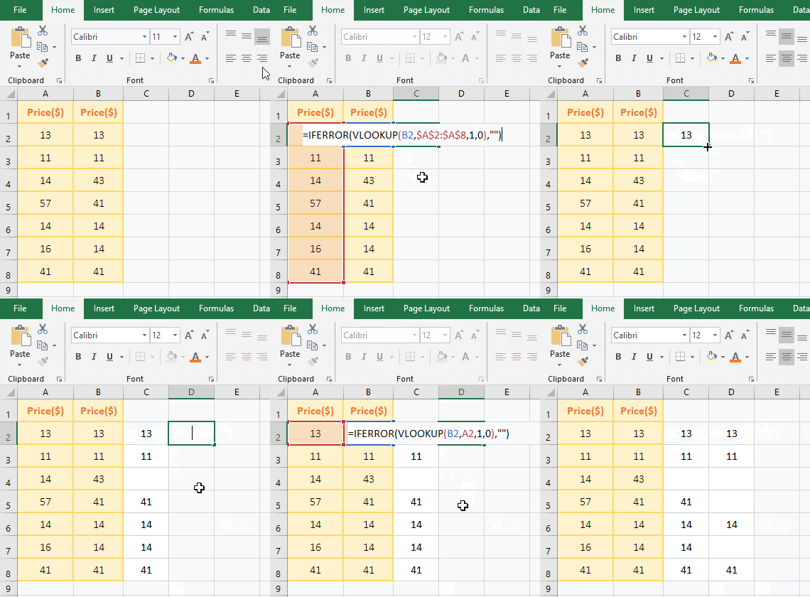
1. If you want to find duplicate values for two columns of prices. Double-click the cell C2, copy the formula =IFERROR(VLOOKUP(B2,$A$2:$A$8,1,0),""), and paste it in C2, press Enter, return to the search result 13, indicating the number of column A Same as the number of the B column in the second row; select the C2 cell, move the mouse to the cell fill handle on the lower right corner of C2, and after the mouse changes to the bold black cross(+), double-click the left button to filter out all price duplicate values og the two columns.

Double-click the cell D2, copy the formula =IFERROR(VLOOKUP(B2,A2,1,0),""), and paste it in D2, press Enter, also return to 13. Use the same method to return the rest of duplicates. Steps as shown in Figure 1:

Figure 1

2. Formula =IFERROR(VLOOKUP(B2,$A$2:$A$8,1,0),"") description

A, B2 is the lookup value of VLookUp, which is a relative reference. Dragging down will change to B3, B4, ...; $A$2 is an absolute reference to the column and row, dragging down will not become A3, A4,... ..., $A$8 and $A$2 are a meaning.

B, $A$2:$A$8 is the range_lookup, which means that B2 is searched from A2 to A8, B2 is changed to B3, B4, ..., and they are also found in A2 to A8.

C, 1 is col_index_num of VLookUp, 0 means exact match; when the formula is in C2, VLOOKUP(B2,$A$2:$A$8,1,0) means to find B2 (ie 13) in A2 to A8, After A2 is found, it returns to the first column of the range_lookup, which returns 13 in column A.

D, IfError is an error return function. If VLOOKUP(B2,$A$2:$A$8,1,0) returns an error value, it returns a null value, otherwise it returns the value that is returned by VLOOKUP(B2,$A$2:$A$8,1,0).

Hint: $A$2:$A$8 can also be represented by a column, ie A:A, but there are two problems with this, one is not supported by a lower version of Excel, and the other is that the execution speed may be slower.

3. The formula = IFERROR (VLOOKUP (B2, $A$2: $A$8, 1, 0), "") and = IFERROR (VLOOKUP (B2, A2, 1, 0), "") difference: the former as long as AB two columns have Duplicate, it will return a duplicate value; the latter will only return values if it is repeated on the same row.

II, How to compare two excel sheets using vlookup

If you want to find the same data in the two tables that are in the "Fruit1.xlsx" and "Fruit2.xlsx" documents, the Sheet name is "Fruit Sale 1" and "Fruit Sale 2", the following is specific Search method:

(I) only require one column with the same data

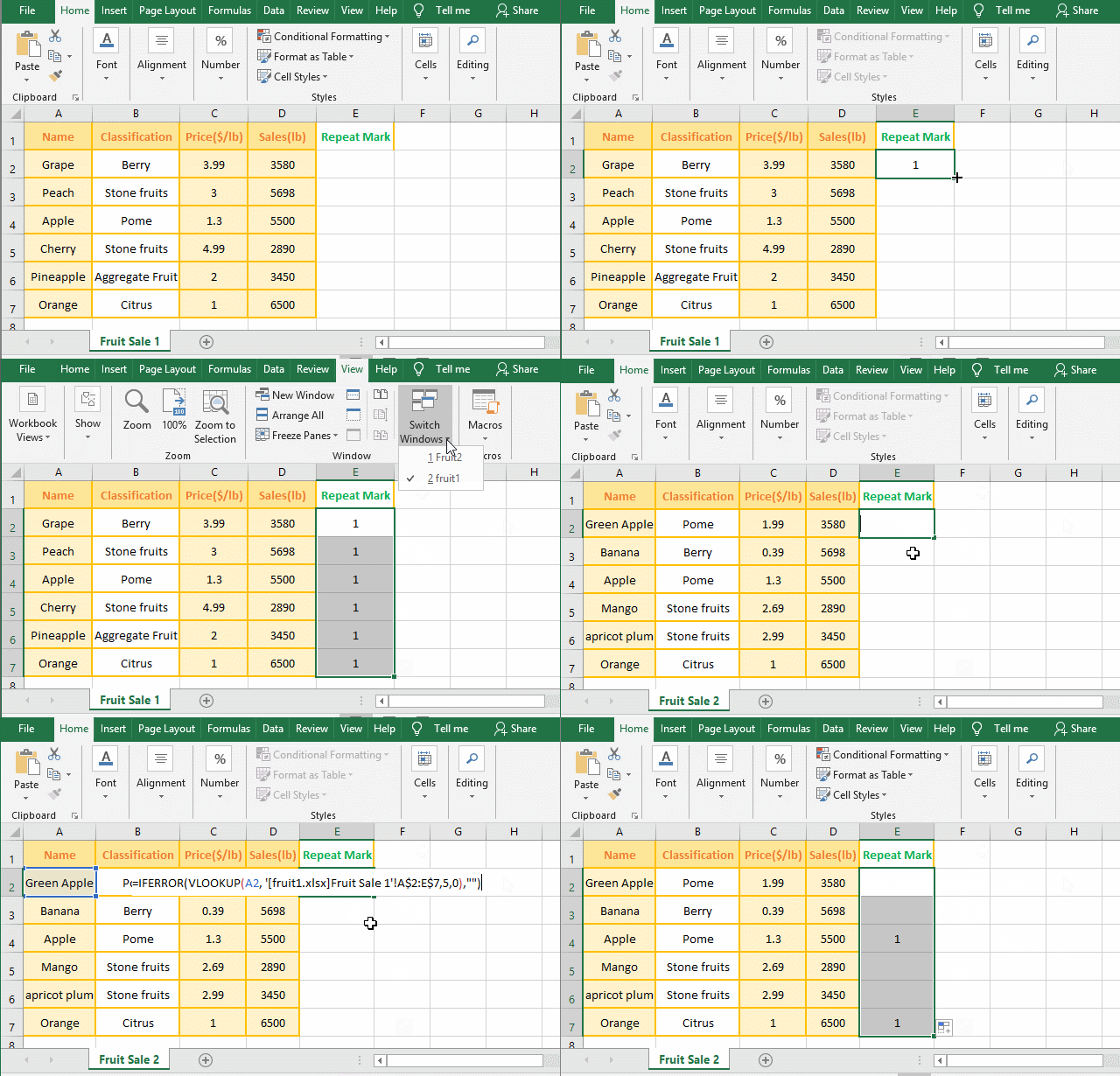
1. In the "Fruit1.xlsx" window, select cell E2, enter 1 and move the mouse to the cell fill handle on the lower right corner of E2. After the mouse changes to the bold black cross(+), double click the left button and the row that include data are Filled in the last column; select the "View" tab, click "Switch Window", select "Fruit2" in the pop-up menu, switch to the "Fruit2" window; double-click cell E2, copy the Formula =IFERROR(VLOOKUP(A2, '[fruit1.xlsx]Fruit Sale 1'!A$2:E$7,5,0),""), and paste it in E2, press Enter, return null, select E2, Move mouse to the cell fill handle on the lower right corner of E2. After the mouse changes to the bold black cross, double-click the left button to return the search result of remainder rows, where the representation of 1 is repeated with the corresponding row of the table in "Fruit1"; Steps as shown in Figure 2:

Figure 2

2. Description:

A. Add 1 in the E column of "Fruit Sale 1" to mark the same data of the two tables in the E column of "Fruit Sale 2", that is, if the two tables have the same data, 1 is showed in the Column E of "Fruit Sale 2".

B. formula =IFERROR(VLOOKUP(A2, '[fruit1.xlsx]Fruit Sale 1'!A$2:E$7,5,0),""), the search value is A2 (A2 of Fruit Sale 2) , the table_array is '[fruit1.xlsx]Fruit Sale 1'!A$2:E$7. Because it is a worksheet in the "Fruit 2.xlsx" to find the worksheet of "fruit1.xlsx", so the table_array must include the document name and worksheet, that is, '[fruit1.xlsx]Fruit Sale 1', and add a half-angle exclamation mark (!) between the work table and the reference cell; 5 is the return column number, that is, return Column 5 of "Fruit Sale 1", ie returns the "Repeat Mark" column.

Tip: If you enter the formula in E2 of "Fruit Sale 2", it is troublesome to enter the document name and worksheet name. After enter =IFERROR(VLOOKUP(A2, switch to the "Fruit1.xlsx" window, click to the sheet name "Fruit Sale 1", it will enter automatically '[fruit1.xlsx]Fruit Sale 1'!, and then select A2:A7, it will enter automatically $A$2:$A$7, switch back to "Fruit2.xlsx", the formula has changed to =IFERROR(VLOOKUP(A2, '[fruit1.xlsx]Fruit Sale 1'!A$2:E$7, then enter other parameters.

(II) Require all columns to have the same data, that is, the data of one row is the same

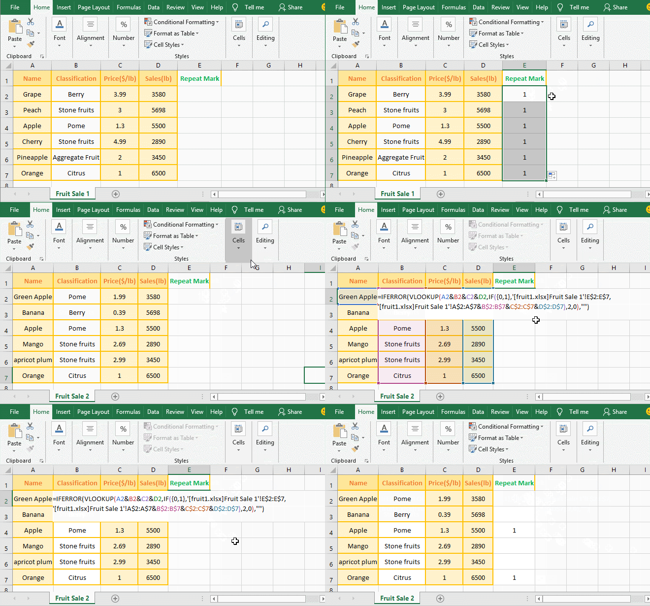
1. It is considered the same if data of two rows are required to be identical. Also add 1 as the repeat marker in the last column of "Fruit Sale 1"; then switch to "Fruit Sale 2", double-click cell E2, and put the formula =IFERROR(VLOOKUP(A2&B2&C2&D2,IF({0,1},'[fruit1.xlsx]Fruit Sale 1'!E$2:E$7,'[fruit1.xlsx]Fruit Sale 1'!A$2:A$7&B$2:B$7&C$2:C$7&D$2:D$7),2,0),"") Copy to E2, press Enter, return null value, then double-click the E2 fill handle to return the remaining search results, display 1 indicates that the row data is the same; operation steps, such as Figure 3 shows:

Figure 3

2. Formula description:

=IFERROR(VLOOKUP(A2&B2&C2&D2,IF({0,1},'[fruit1.xlsx]Fruit Sale 1'!E$2:E$7,'[fruit1.xlsx]Fruit Sale 1'!A$2:A$7&B$2:B$7&C$2:C$7&D$2:D$7),2,0),"")

A. A2&B2&C2&D2 are the lookup_value, which are the data of the four cells A2, B2, C2, and D2, that is, "Green ApplePome1.993580".

B. IF({0,1},'[fruit1.xlsx]Fruit Sale 1'!E$2:E$7,'[fruit1.xlsx]Fruit Sale 1'!A$2:A$7&B$2:B$7&C$2:C$7&D$2:D$7) is to list the data  that is Per Row of the table_array A:D in the "fruit sale 1" as a column and the return column E as a separate column; if you do not understand, please refer to "Vlookup with if statement(use if/if{0,1} combination two or three conditions)" article, which has a detailed explanation.

Tip: If you only need two tables, two columns or three columns have the same data, for example, only A, B, and C columns are required to have the same data, just keep A2, B2, and C2 consecutive, that is, A2&B2&C2.