The use instances of Excel Round function, include Round a number to two decimal places

The Round function in Excel is used to round a number to a specified number of digits. It is divided into three cases, namely, round a number to a specified number of digits, round a number to the nearest integer, and round a number to the left of the decimal point. There is an advantage to using the Round function, that is, only the decimal are rounded to the specified number of digits, and the integer returns itself, which avoids ".0".

In daily work, the Round function is used generally to round the calculated result to the specified number of digits when averaging or dividing, because their calculated results are rounded automatically different decimal places based on the size of the operand. In addition, if you do not use the Round function when calculating with a formula, you can increase the formula in batches.

I, The syntax of the Excel Round function

1. Expression: ROUND(Number, Num_Digits)

2. Description:

A. If Num_Digits is greater than 0, round the number to the specified number of decimal places; if Num_Digits is equal to 0, round the number to the nearest integer; if Num_Digits is less than 0, round the number to the nearest digit to the left of the decimal point.

B. There are three functions similar to the Round function, namely the RoundUp function, the RoundDown function, and the MRound function; RoundUp is used for rounding up, RoundDown is used for rounding down, and MRound is used to round the number to a specified multiple.

II, The use instances of Excel Round function

(1) Round a number to two decimal places

1. Select cell B2, enter the formula =round(a2,2), press Enter, return to round 6.324 in A2 to the result 6.32; select B2, move the mouse to the cell fill handle on the lower right corner of B2, double-click the left button after the mouse becomes bold black plus, the remaining values are rounded automatically two decimal places; the operation steps, as shown in Figure 1:

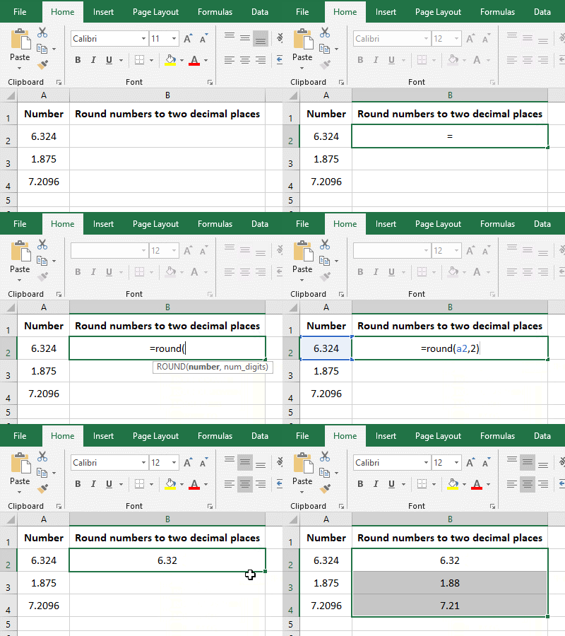
Figure 1

2. In the formula =round(a2,2), 2 is the number of two decimal places; as can be seen from the demo, the values that were rounded two decimal places are rounded, such as 6.324 to 6.32, 1.875 became 1.88.

(2) Round a number to a nearest integer

1. If it is required to round the "monthly average sales" to nearest integers. Double-click the cell G2, copy the formula =ROUND(F2,0), and paste it in cell G2, press Enter, and return to the result 404. Also double-click the fill handle of cell to round the remaining values to nearest integers; the operation steps are as shown in Figure 2:

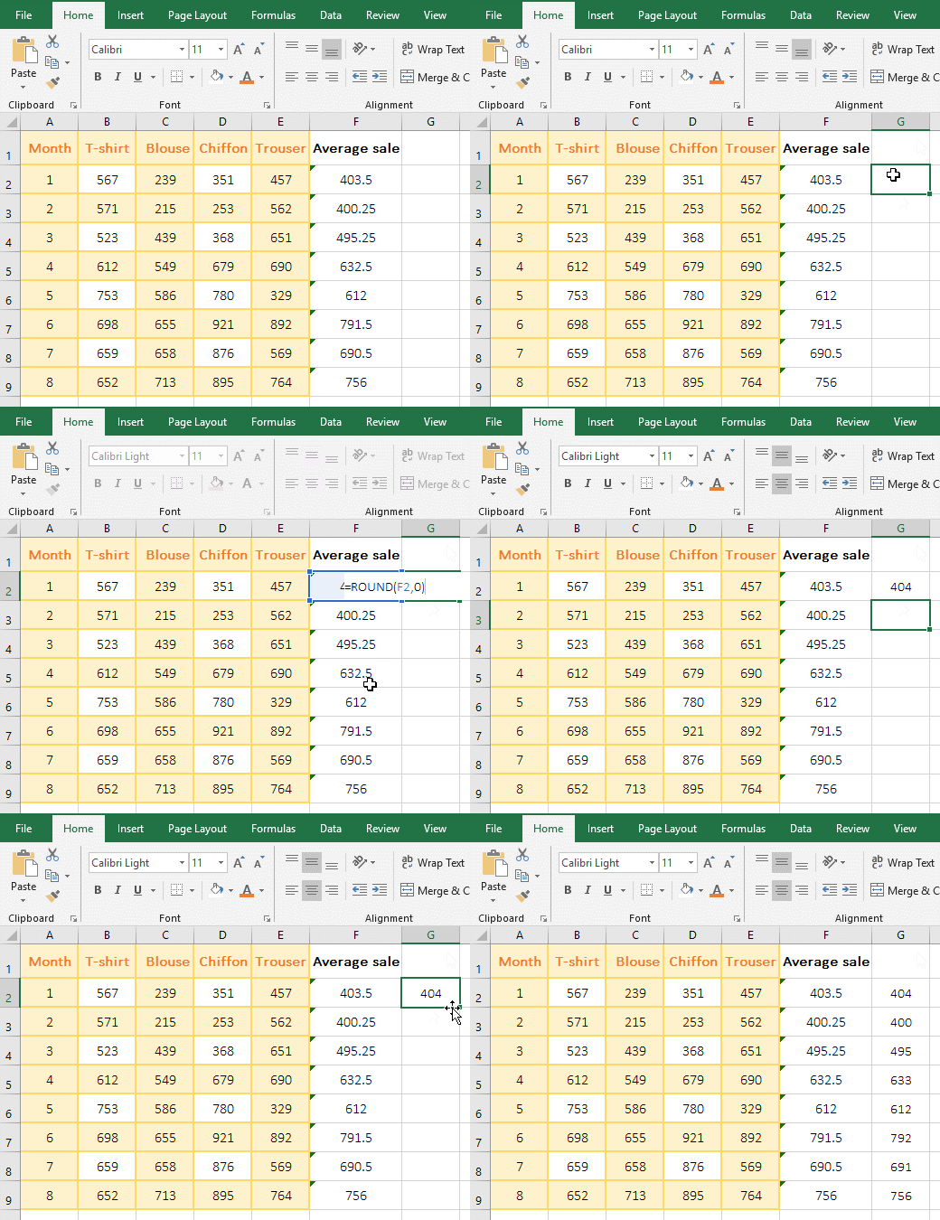
Figure 2

2. In the formula =ROUND(F2,0), 0 means to round a number to a nearest integer; from the returned result, they are rounded off by the Round function.

(3) Round the number to the nearest digit to the left of the decimal point

(1) The number of rounded digits is an integer

1. Select cell B3, enter the formula =round(a3,-1), press Enter, return to 460; move the mouse to the fill handle on the lower right corner of cell B3, after the mouse changes to the bold black plus sign, double-click the left button to round the remaining value to the nearest digit to the left of the decimal point. Select C3, enter the formula =round(a3,-2), press Enter, return to 500, and double-click the fill the handle of C3 to return the results of the remaining value; select D3, enter the formula =round (a3, -3), press Enter, return 0, and then use the method of double-clicking the fill handle of cell to return the results of other values; the operation steps, as shown in Figure 3: :

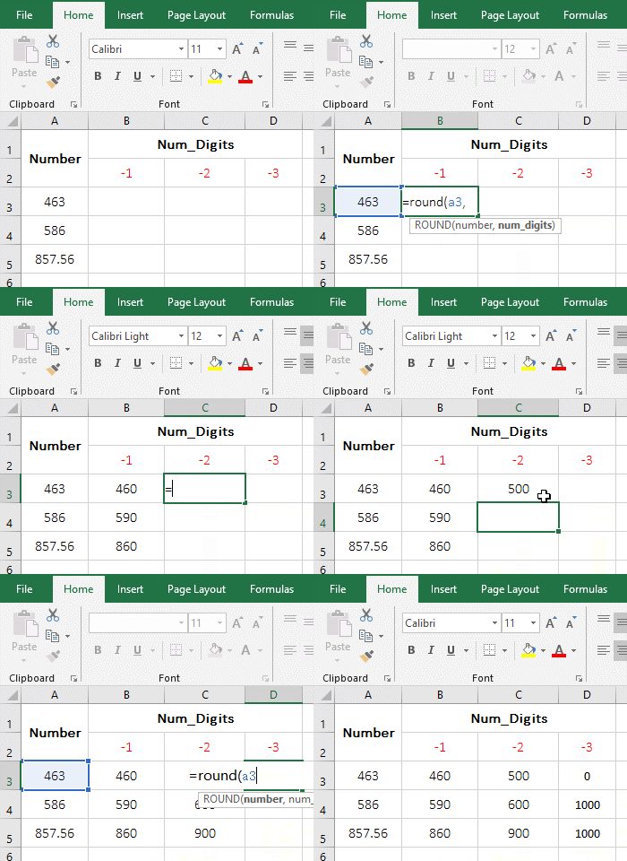
Figure 3

2. Formula description:

A. In the formula =round(a3,-1), -1 means rounding the value in a3 to the left of the decimal point by 1 digit, that is, the digits are rounded to the ten digits. 463 in a3 becomes 460, 3 is discarded; 586 becomes 590, the ten's place 8 increase by 1, the unit's digit 6 is discarded, and 8 liters to 9; 857.56 becomes 860, and the ten's place 5 increase by 1.

B. In the formula =round(a3,-2), -2 means rounding the value in a3 to the left of the decimal point by 2 digits, that is, the ten digits are rounded to the hundred digits. 463 becomes 500, the hundred's place 4 increase by 1, the ten's place and the unit's digit are discarded; others and so on.

C. In the formula =round(a3,-3), -3 means rounding the value in a3 to the left of the decimal point by 3 digits, that is, the hundred digits are rounded to the thousand digits. 463 becomes 0, because the 4 of the hundred digits are less than 5, do not carry 1 to thousands; 586 becomes 1000, the 5 of the 100 digits carry 1 and the hundreds digits become 0, and the ten digits and the unit's digits are leaved out; others and so on.

(2) The number of rounded digits are decimals

1. Select cell B3, enter the formula =round(a3,-2.4), press Enter, return to 500, and double-click the fill handle of cell B3 to return the result of the remaining values; Select C3 and enter the formula =round(a3, -2.5), press Enter, also return to 500; the operation steps, as shown in Figure 4:

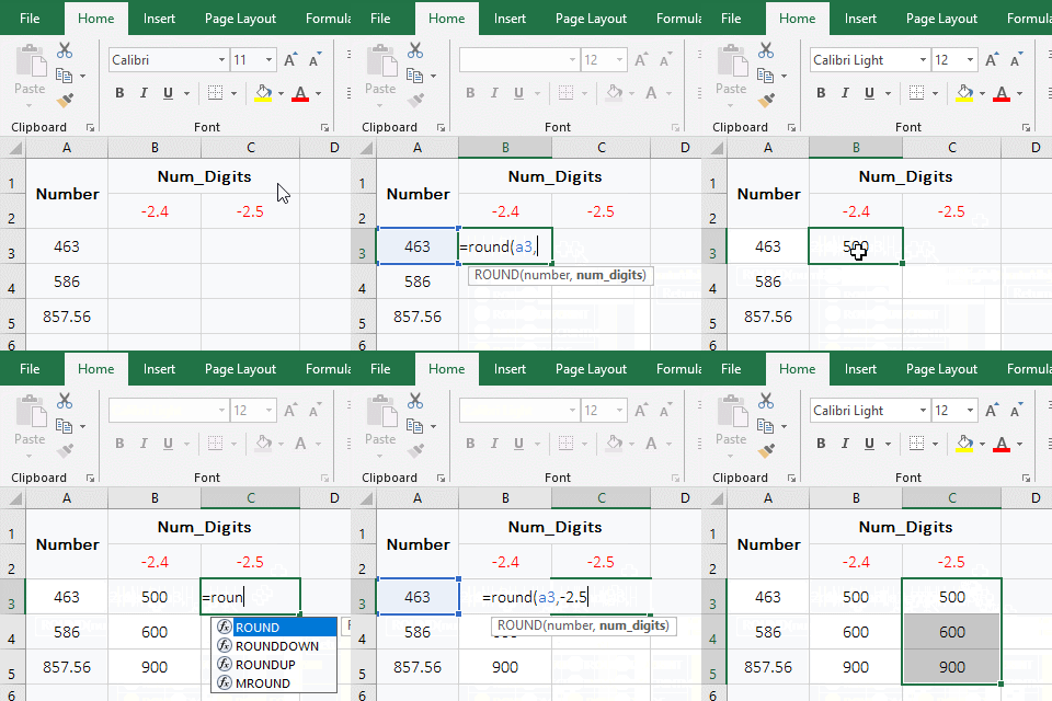
Figure 4

2. Formula description:

The formula =round(a3,-2.4) returns the same result as =round(a3,-2.5), indicating that if the "Num_Digits" is a decimal, the fractional part is not rounded off, but it is discarded directly.

III, The application examples of Excel Round function

(1) Round + Average function return integers after Averaging

1. If the average sales of various clothing is required every month, no decimals are required. Double-click cell F2, copy the formula =ROUND(AVERAGE(B2:E2),0), and paste it in F2, press Enter, return to the averaged result 404; return the average sales of the remaining months with the double-click the fill handle of cell. The process steps are shown in Figure 5:

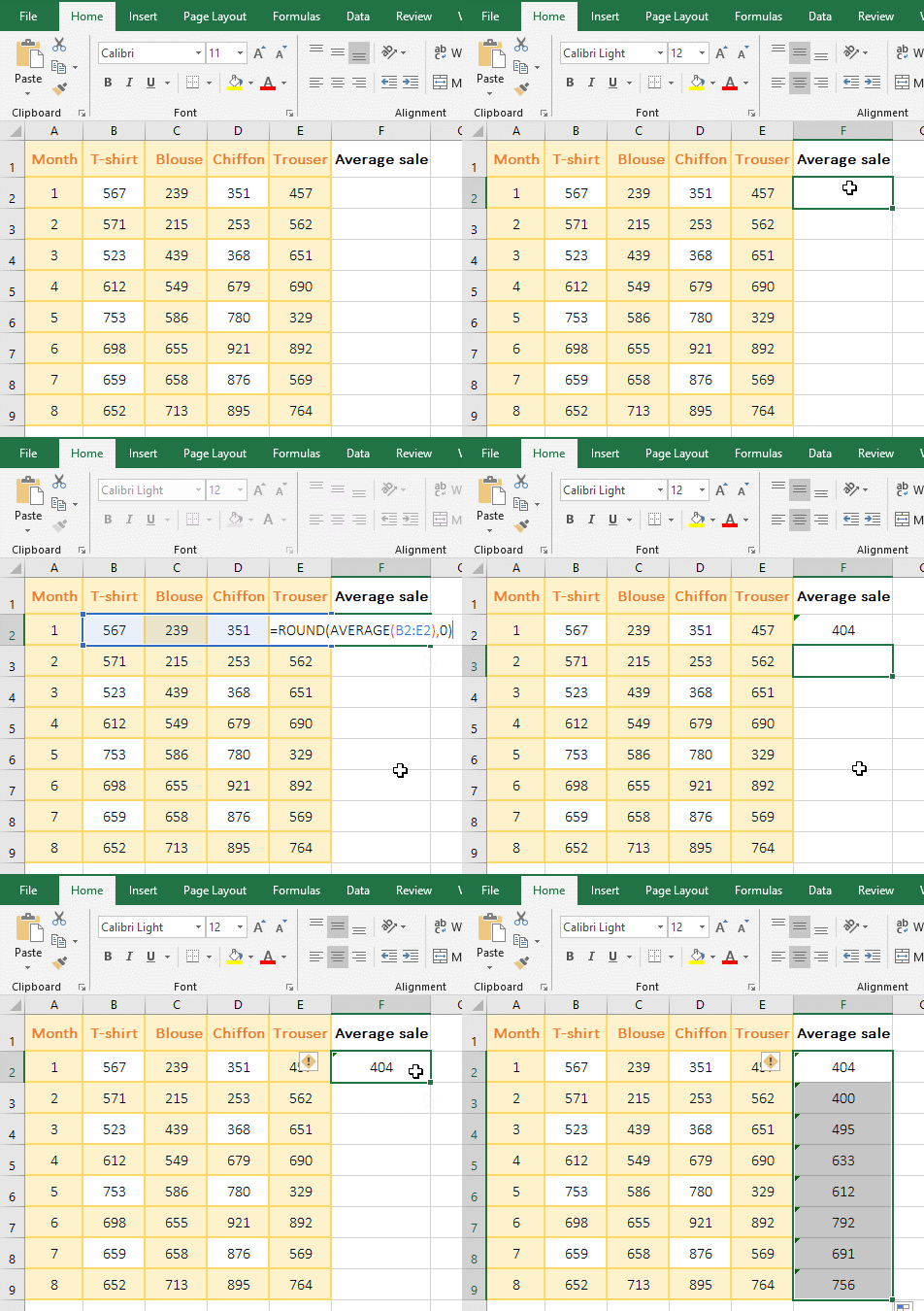
Figure 5

2. Formula =ROUND(AVERAGE(B2:E2),0) description:

AVERAGE(B2:E2) is used to calculate the average of B2 to E2, which returns 403.5; the formula becomes =ROUND(403.5,0), and finally rounded up, the result is 404.

(2) Round the integers to 0 dicimal place, round the decimals to two decimal places

1. If you are required to calculate the salary, and the results are rounded 1 decimal place. Double-click cell F2, copy the formula =ROUND(SUM(D2:E2),1), and paste it in F2, press Enter, return to 4723.6; double-click the fill handle of cell F2 to return the salary of the remaining employees. The process steps are shown in Figure 6:

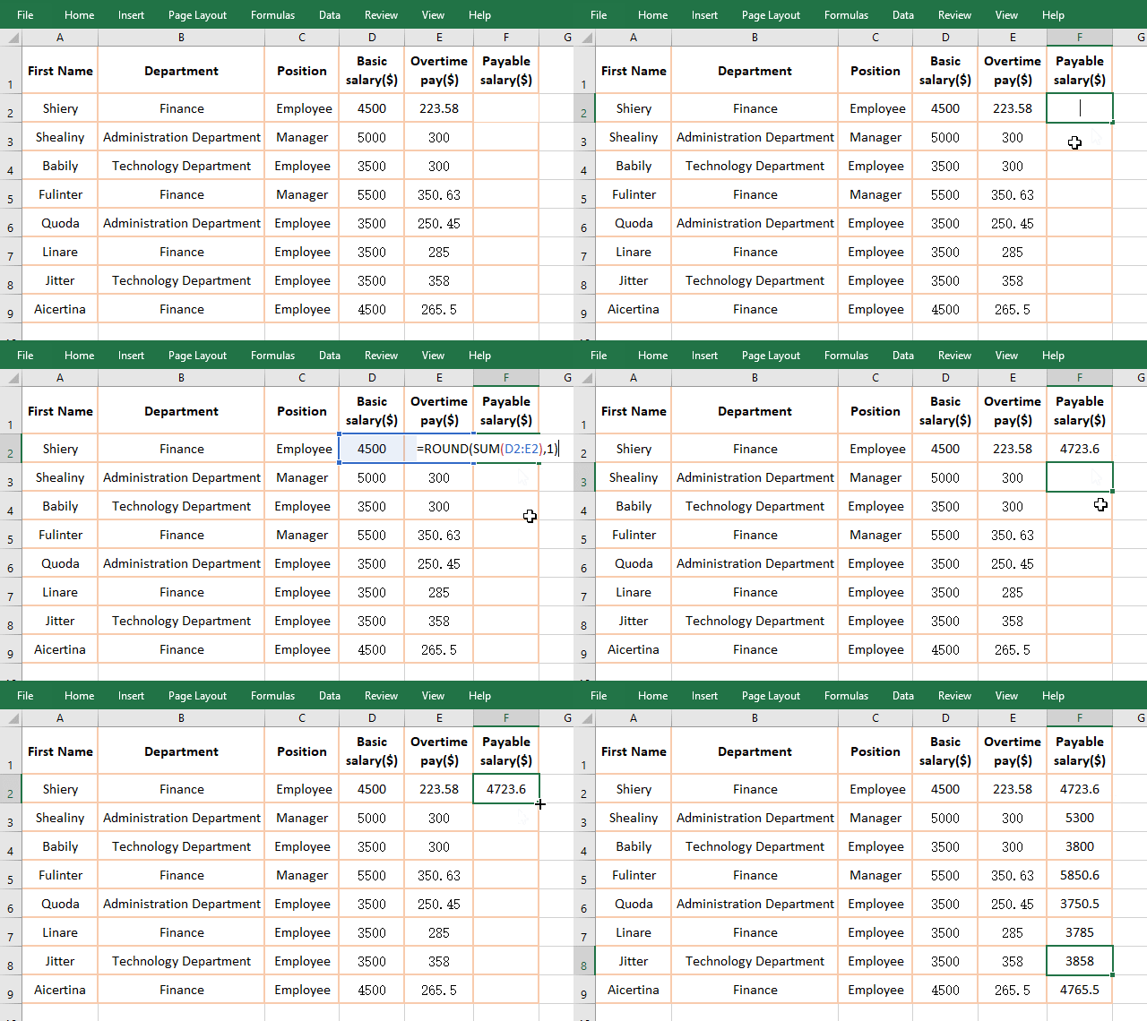
Figure 6

2. Formula =ROUND(SUM(D2:E2),1) explanation:

SUM(D2:E2) is used to return the sum of "Basic Salary" and "Overtime Pay", and then round the result of the sum to 1 decimal place; from the operation, the summation result that is decimal is rounded to, such as 4500 + 223.58 = 4723.6; Only integers are rounded, such as 5000 + 300 = 5300.

(3) Add the Round function to the existing formulas in batches.

There is a table that has calculated the average monthly profit, but does not round the values to two decimals. Now you need to use the Round function to do this, as follows:

1. Press the shortcut keys Ctrl + ~ to display the formulas, press Ctrl + H, open the "Find and Replace" dialog box and select automatically the "Replace" tab, then replace the three items separately, as follows:

A. Replace "=" with "-=". Enter = on the right side of "Find what", enter "-=round" on the right side of "Replace with", click "Options" to expand, select "sheet" for "Within", select "Formula" for "Look in", click "Replace All", pop-up a dialog box that prompt "All done. We made 8 replacements".

B. Replace after the formula brackets "(" with "), 2)". Enter the half-width brackets on the right side of "Find what", enter ")" on the right side of "Replace with ", 2), click "Replace All", and also prompt "All done. We made 8 replacements".

C. "-=" replace back "=". Enter "-=" to the right of "Find what", enter "=" on the right side of "Replace with", click "Replace All", and also prompt "All done. We made 8 replacements", then all formulas are batched with Round, click "Close" to close "Find and Replace" window; the operation steps are as shown in Figure 7:

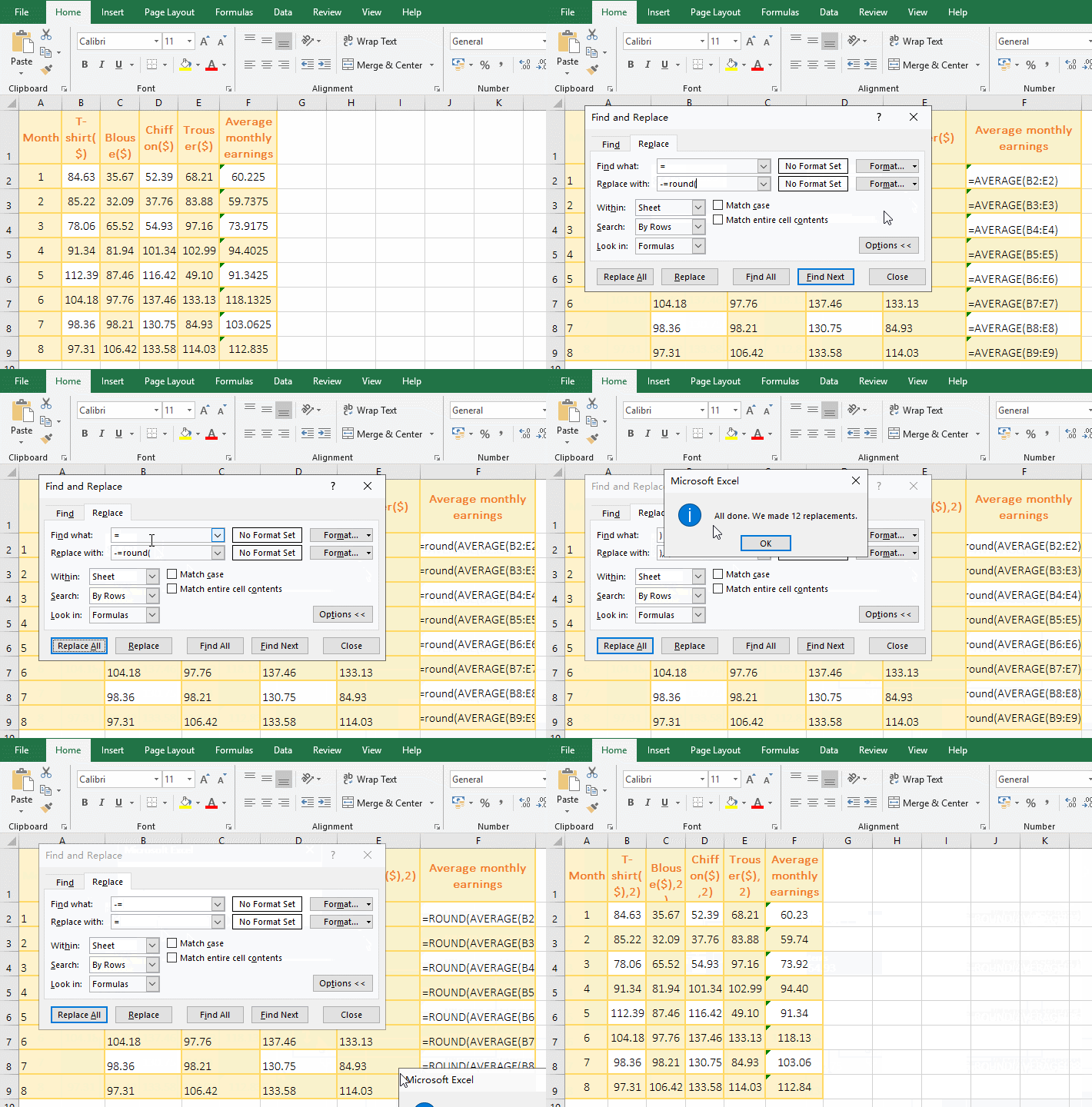
Figure 7

2. Description:

Because replace directly "=" with "=round(", there will be a formula that does not conform to the syntax and prompt an error, so first replace "=" with "-=round(" that is, first convert the formula to text, replace it and then replace "-=" by "=" again, that is, restore the text to a formula.