VLookUp in excel introduces step by step(10 examples), include Reverse lookup,one-to-many lookup

The VLookUp in excel is a function for finding a specified value by row; it has at least three parameters, and the fourth parameter is an option to determine the matching option (exact match or approximate match). If it is left out, the default is approximate match. The VLookUp function involves a lot of lookups. If the settings are incorrect, you may return multiple error values.

The VLookUp function is used in a lot of ways. This article will introduce its syntax, basic usage and common methods.The basic usage describes six examples, the common methods introduce three instances. The examples contain multiple returnerror values, and use wildcard questions mark (?) and asterisks (*), and reverse lookups, and approximate matches, and one-to-many lookup.

I, Syntax of VLookUp in excel

1, Expression: VLOOKUP (LookUp_Value, Table_Array, Col_Index_Num, [Range_LookUp])

2, Description

(1), Col_Index_Num takes the left-most column of Table_Array as the first column. For example, if the specified rangeis B2:D8, the column B is the first column; if Col_Index_Num is set to 2, the value of column C is returned.

(2) Range_LookUp is an optional parameter. It has two options, one is True, the other is False, True is an approximate match, False is an exact match, and if Range_LookUp is left out, True is selected by default.

(3) Common return errors

A. If Range_LookUp is set to True (approximate match), the first column of Table_Array needs to be sorted, otherwise the error value may be returned; if Range_LookUp is set to True, LookUp_Value is smaller than the smallest value of the first column in Table_Array, and the error value #N/A will be returned; If Range_LookUp is set to False, if the error value #N/A is returned, there is no lookup value in Table_Array.

B. If Col_Index_Num is greater than the number of columns in Table_Array, the reference error value #REF! will be returned.

C. if Table_Array is less than 1, it will return the value error #VALUE!.

D. If the formula is missing quotes, it usually returns the name error value #NAME?.

(4) When searching for numbers or dates, the first column of Table_Array cannot be set to text, otherwise incorrect values may be returned.

(5) If Range_LookUp is set to False (exact match) and LookUp_Value is text, you can use the wildcard question mark (?) and asterisk (*) in LookUp_Value; the question mark represents any character, and the asterisk indicates one or more characters. If you want to find the question mark or asterisk, you need to add the escape character ~ in front of them, for example, to find the question mark(?), it should be like this ~?.

(6) There must be no spaces, or single and double quotation marks, or non-printing characters in Table_Array. If there are these characters, they should be removed by function or replacement. Otherwise, unexpected values may be returned.

II, Usage and examples of VLookUp in excel(VlookUp step by step)

(I) Parameter Range_LookUp is left out

1. If you want to find the "sales" of "Pink Shirt". Select cell A11, copy the formula =VLOOKUP("Pink shirt",A2:D10,4,), and paste it in cell A11, press Enter, return to the search result 892; the operation steps are as shown in Figure 1:

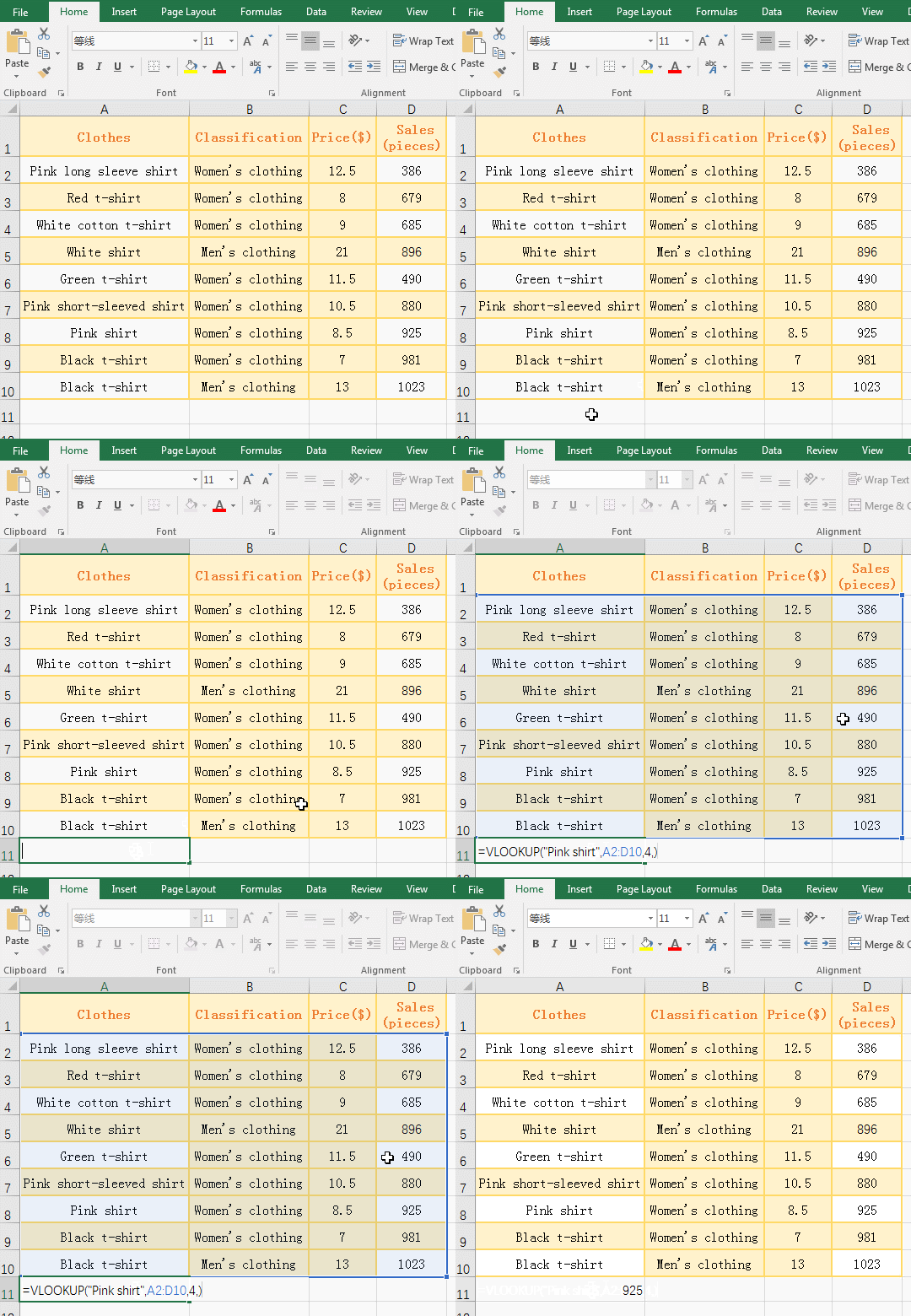
Figure 1

2. Formula description:

A. "Pink shirt" is the lookup value in the formula =VLOOKUP("Pink shirt",A2:D10,4,), A2:D10 is Table_Array, and 4 is the return column number (that is the column A is the first column of Table_Array, and the fourth column is returned, that is the value of column D), the formula is left out the fourth parameter Range_LookUp, the default is True (approximate match). The formula means: look for "Pink shirt" in Table_Array B2:E8, and return the value in D8 that is corresponding with A8 after A8 is found in column A, that is, returns 892.

B. If the fourth parameter Range_LookUp is left out, there are both comma (,) and comma (,) can be left out after the third parameter in fourth.

(II) Set the parameter Range_LookUp to True, the first column of Table_Array needs to be sorted alphabetically or numerically, and LookUp_Value is less than the smallest value of the left-most column of Table_Array will return #N/A

1. Double-click cell B13, copy the formula =VLOOKUP(A13,C2:D10,2,TRUE), and paste it in cell B13, press Enter, return the error value #N/A; select C2:C10, and select the "Data" tab, click the "Sort A to Z" icon, open the "sort Warning" window, select "expand the selection", click "Sort", then each line is ordered by "price" "smallest to largest", the value in B13 becomes 981. Select cell A13, enter 5, click B13, then the value in B13 becomes the error value #N/A; the operation steps are as shown in Figure 2:

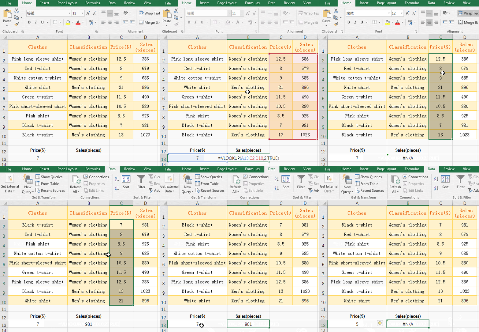
Figure 2

2. Formula description:

A. Formula =VLOOKUP(A13,C2:D10,2,TRUE) Set the parameter Range_LookUp to True, return the error value #N/A before sort by the "Price", and sorted by the "price" "smallest to largest", can return the correct lookup value 981, indicating that when the parameter Range_LookUp is set to approximate match, the first column of Table_Array needs to be sorted to ensure that the correct lookup value is returned.

B. The first column of Table_Array can be sorted. If the lookup value(5) is smaller than the smallest value(7) of the left-most column of Table_Array, the error value #N/A is also returned.

(III) Set the parameter Range_LookUp to False to return error value #N/A

1. Double-click cell B13, copy the formula =VLOOKUP(A13,C2:D10,2,FALSE), and paste it in cell B13, press Enter, return the error value #N/A; the operation procedure is as shown in Figure 3:

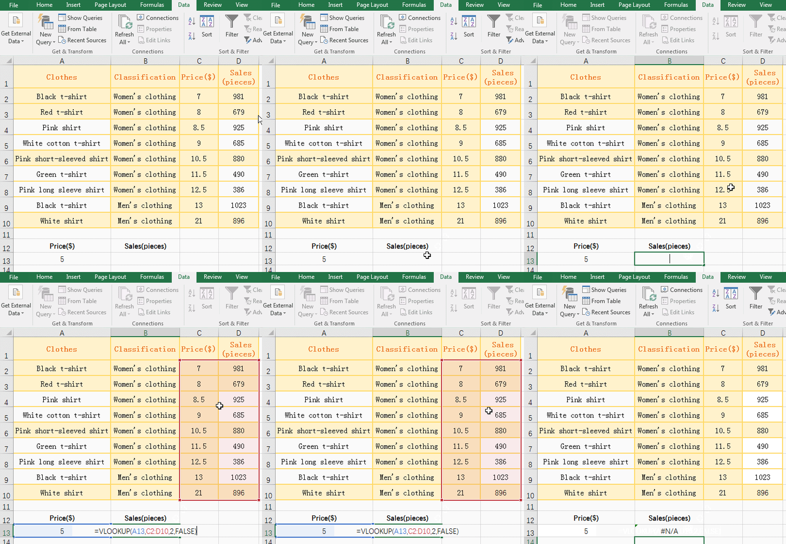
Figure 3

2. When the parameter Range_LookUp is set to False (exact match), Whether to sort the left-most column of Table_Array, and if no value is found, the error value #N/A is returned.

(IV) The formula is missing quotes to return the name error value #NAME?

1. Double-click cell B13, copy the formula =VLOOKUP(Black t-shirt,A2:D10,4,FALSE), and paste it in cell B13, press Enter, return the name error value #NAME?; double-click B13, to enter double quotation marks the "black t-shirt" each side in the formula, press Enter, return to find value 981; operation steps, as shown in Figure 4:

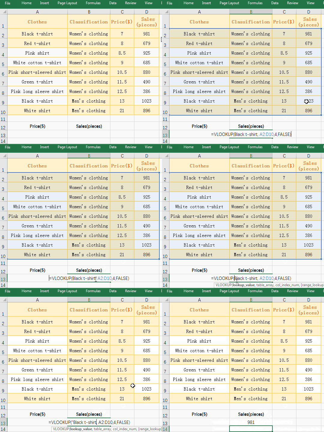
Figure 4

2. If Look_Value is the text, it must be enclosed in double quotation marks, otherwise it returns the name error value #name?.

(V) Use wildcard question mark (?) or asterisk (*) in the LookUp_Value

(1) Use question mark (?) in the LookUp_Value

1. If you look for the "Clothes" property starting with "Pink" and only six characters after "Pink", and look for "Clothes" property that is only question mark(?). Double-click cell B13, copy the formula =VLOOKUP(A13,A2:D10,4,), and paste it in cell B13, press Enter, return to the search result 925. Double-click cell A13, change the content to ~?, click B13,  the value in B13  becomes 490; the operation steps are as shown in Figure 5:

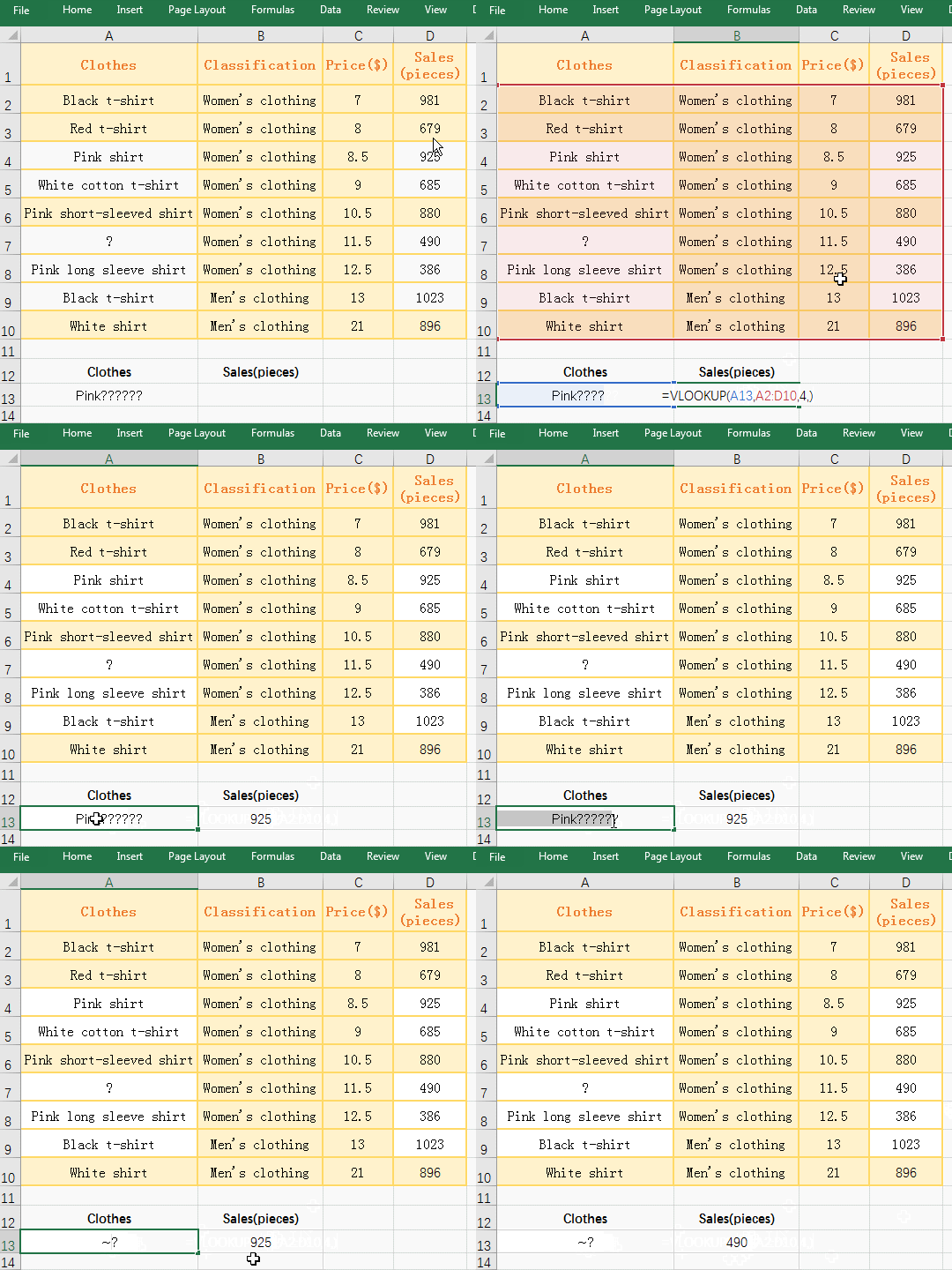
Figure 5

2. Description:

A. "Pink??????" in A13 means start with "pink" and only six characters behind it, it happens to be "pink shirt", clothing property of A6 and A8 also start with "Pink", but there are more than six characters after "Pink", so the conditions are not met.

B. Change the content of A13 to ~?, indicating that you want to find the question mark, just return ? corresponding sales 490.

(2) Use asterisk (*) in the Lookup_Value

1. If you look for "Clothes" property begin with "pink", or end with "t-shirt", or begin with "white" and end with "shirt". Double-click cell B13, copy the formula =VLOOKUP("Pink*", A2:D10,4,), and paste it in cell B13, press Enter, return to the search result 329; double-click B13, change the Lookup_Valu "Pink*" to "*t-shirt", press Enter, return to find result 981; double-click B13, change the Lookup_Value "*t-shirt" to "white*shirt", press Enter, return to the search result 685; the operation steps, as shown in Figure 6:

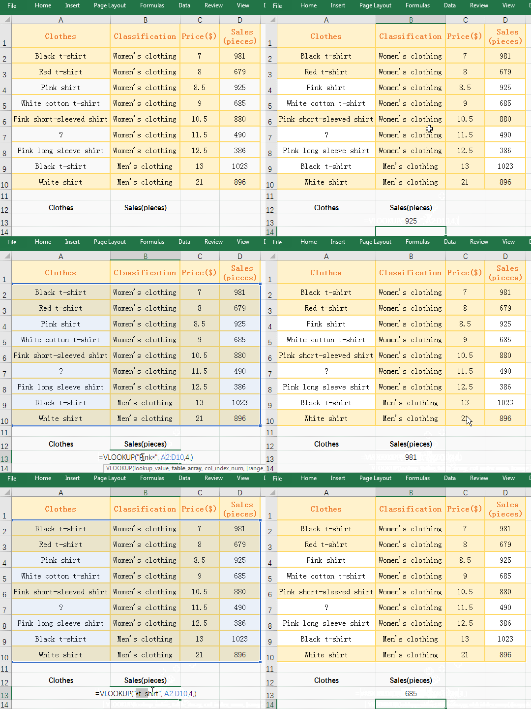
Figure 6

2. Description:

Formula = VLOOKUP ("Pink*", B2:E8,4,) "Pink*" means finding clothing starting with "Pink", *T-shirt" means finding clothing that starts with any character and ends with "T-shirt" , white * shirt "represents the look for clothing that begins with "white" and ends with "shirt."

(VI) Parameter Table_Array has spaces before and after

1. If you want to find the "green T-shirt" in A11. Double-click cell B13, copy the formula =VLOOKUP(A13,A2:D10,4,), and paste it in cell B13, press Enter, return the error value #N/A; double-click B13 and change the formula to =VLOOKUP(A13,TRIM(A2:D10),4,), press Ctrl + Shift + Enter to return to the search value 490; the operation steps are as shown in Figure 7:

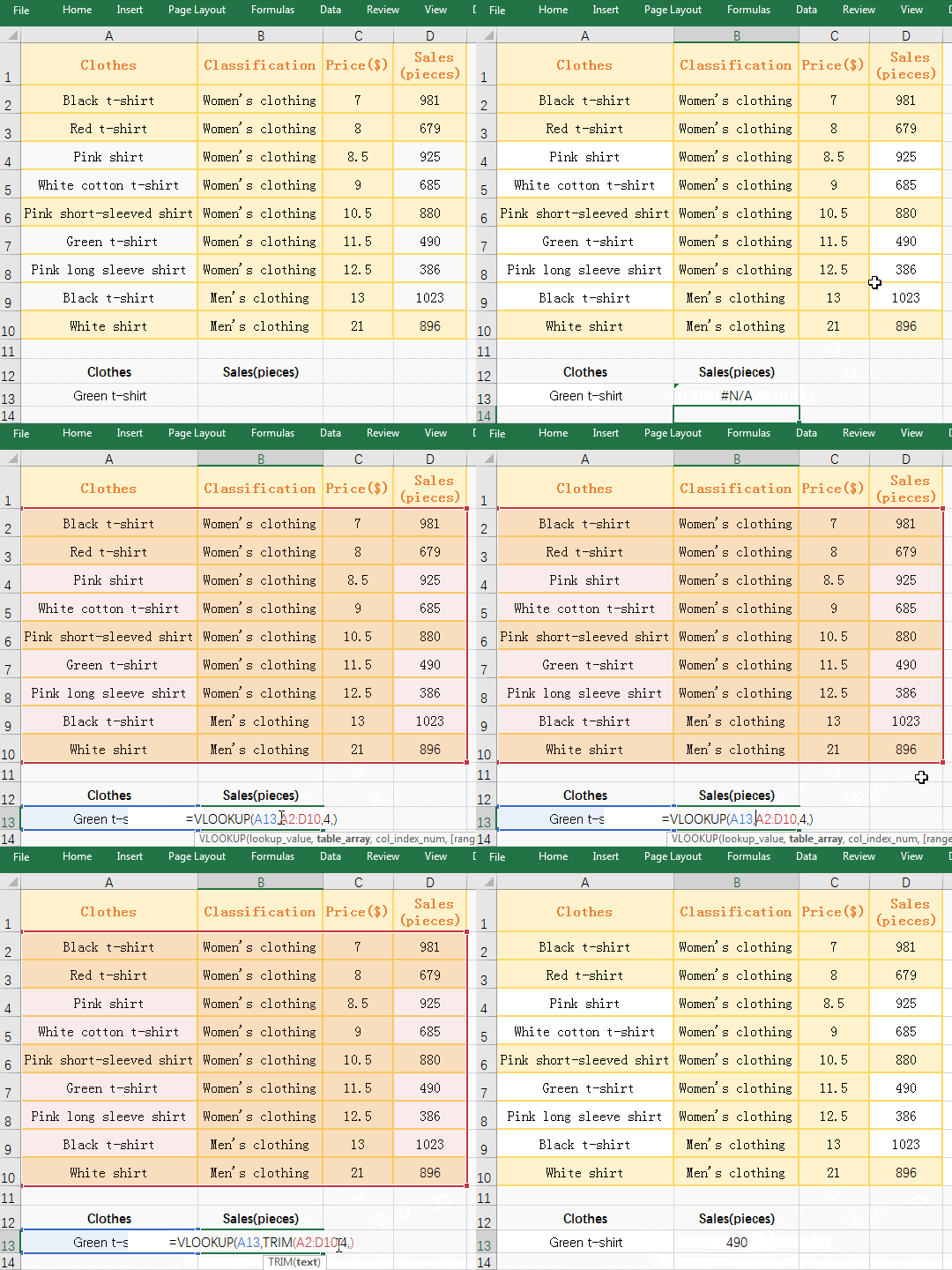
Figure 7

2. Formula description:

A. The contents of A7 are "Green t-shirt", but the formula =VLOOKUP(A13,A2:D10,4,) returns the error value #N/A, and the space before and after are removed after add the function Trim, and the correct value can be returned, indicating that there are space in A7.

B. =VLOOKUP(A13,TRIM(A2:D10),4,) is an array formula, so you need to press Ctrl + Shift + Enter, because A2:D10 returns all the values in A2:D10 as an array, then use Trim function removes the spaces one by one.

III, VLookUp in excel is used in common examples(VlookUp step by step)

(I) Approximate matching

1. If you want to find the student's Grade that based on the average score. Select cell G9, enter =a5, press Enter, return to "Bulen"; double-click H9, copy formula =VLOOKUP(E5,G3:H6,2), and paste it in cell G9, press Enter, return to Bulen's Grade B; process steps, as shown in Figure 8:

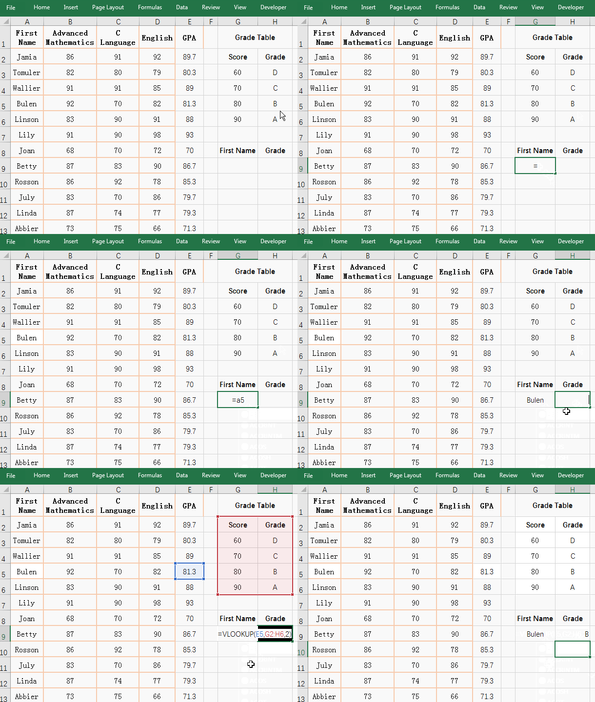
Figure 8

2. Formula description:

A. Formula =VLOOKUP(E5,G3:H6,2) means to find the Bulen's average score in G3:H6(Grade Table), if found, return the corresponding Grade, since the number in E5 is 81.3, this value is not available in the Grade Table, so an approximation of the 80 to 89 segment can only be selected with an approximate match (ie, the parameter Range_LookUp is left out or set to True).

B. Tip: The scores in the Grade Table must be sorted in ascending order, otherwise incorrect values may be returned.

(II) Reverse lookup(VLookUp + Choose)

1. If you want to find the corresponding "Product code" according to "Clothes". Double-click cell C13, copy the formula =VLOOKUP(B13,CHOOSE({2,1},A2:A10,B2:B10),2), and paste it in cell B13, press Enter, return to "Product code" property WS-581; Operation procedure As shown in Figure 9:

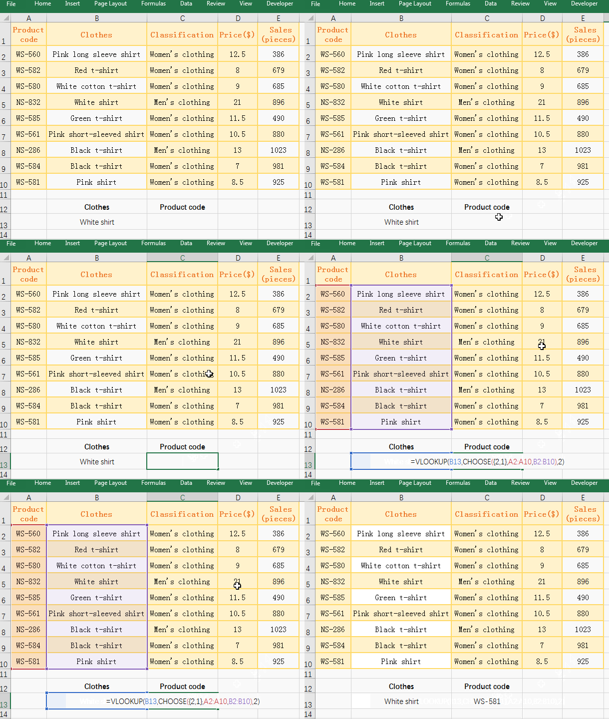
Figure 9

2. The formula =VLOOKUP(B13,CHOOSE({2,1},A2:A10,B2:B10),2) Description:

A. {2,1} are the index_num that are an array in the Choose function to specify which value to return. A2:A10 and B2:B10 are the return values, 2 in the array represents the value in A2:A10, and 1 in the array represents the value B2:B10. When executed, first take 2 out of the array, then take B2 from B2:B10(ie "Pink long sleeve shirt") and take A2 out of A2:A10(ie "WS-580"), Finally, these two elements are grouped into the first element of array, namely "Pink long sleeve shirt", "WS-560"; the second time B3:B10 is taken out of B3(ie "Red t-shirt") and Take A3(ie "WS-582") from A2:A10, form the second element of the array "Red t-shirt", "WS-582"; Finally return the array {"Pink long sleeve shirt", "WS-560"; "Red t-shirt", "WS-582"; "White cotton t-shirt", "WS-580"; "White shirt", "NS-832"; "Green t-shirt", "WS-585"; "Pink short-sleeved shirt", "WS-561"; "Black t-shirt", "NS-286"; "Black t-shirt", "WS-584"; "Pink shirt", "WS-581"}, so put the "Clothes" property in front of the "Product code" property.

B. the formula becomes =VLOOKUP(B13,{"Pink long sleeve shirt", "WS-560"; "Red t-shirt", "WS-582"; "White cotton t-shirt", "WS-580"; "White shirt", "NS-832"; "Green t-shirt", "WS-585"; "Pink short-sleeved shirt", "WS-561"; "Black t-shirt", "NS-286"; "Black t-shirt", "WS-584"; "Pink shirt", "WS-581"},2), after finding the A11 (black T-shirt),  return to the second column, which happens to be WS-581.

(III) one-to-many lookup

1. If you want to find the First Names of all employees of the designated "department"(Sales department). Double-click cell F2, enter "Sales department", double-click A2, copy the formula =(C2=$F$2) + A1, and paste it in cell A2, press Enter, return to 0; Select A2 again, move the mouse to the cell fill handle on the lower right corner of A2, after the mouse becomes the black plus sign (+), double-click, A3 to A8 are all filled with the corresponding numbers. Double-click G2, copy the formula =IFERROR(VLOOKUP(ROW(A1),A1:C$8,2,0),""), and paste it in cell G2, press Enter, return to find the result is "Jaik", select G2, move the mouse to the cell fill handle pn the lower right corner of G2, hold down the left button, drag down, drag until the last row, then return to all employees of the "Sales department". Then double-click C2, Select "Finance", double-click G2 , change "sales department" to "Finance", press Enter, return to the names of all employees of the "Finance department"; the process steps, as shown in Figure 10:

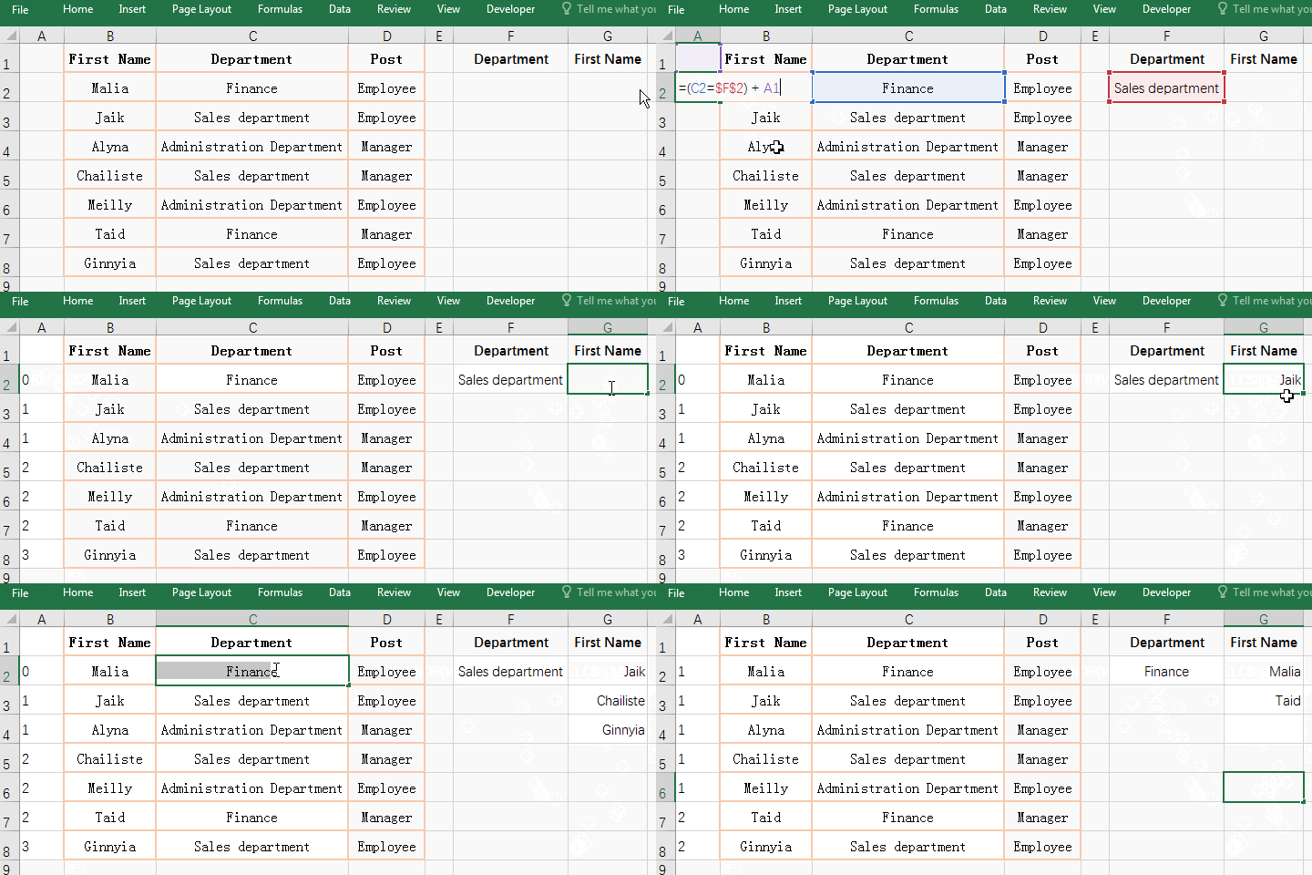
Figure 10

2. Formula description:

(1)=(C2=$F$2)+A1

A. Formula = (C2 = $ F $ 2) + A1 is used to increment the number of employees belonging to the same department, for example, three employees belonging to the "Sales Department" are numbered 1, 2, 3, belonging to the "Finance department" Both employees are numbered 0 and 2.

B. C2 means that the column and the row are relative references. When drag down, it will change to C3, C4, ...; when dragged to the right, it will become D2, D3, .... $F$2 means that the column and the row are absolute references. When you drag down or to the right, F2 does not change.

C. C2=$F$2 is a condition, that is, if C2 is equal to F2, it will return True, otherwise it returns False, and content of C2 is "Finance",  and content of F2 is "Sales department", they are not equal, so it returns True. Then the formula =(C2=$F$2)+A1 becomes =FALSE+A1. When calculating, FALSE is converted to 0, A1 is empty, and 0 is returned by default, so =TRUE+A1 returns 0.

D. Drag down to A3, C2 becomes C3, A1 becomes A2, so the formula of A3 is =(C3=$F$2)+A2; the value of C3 is "Sales Department", equal to F2, so return True, the value of A2 is 0, so the formula becomes =1+0. Since True is converted to 1 when calculated, =1+0 returns 1.

(2) =IFERROR(VLOOKUP(ROW(A1), A1:C$8,2,0),"")

A. ROW(A1) returns the row number 1 of A1; A1:C$8 means the cell range that is from A1 to C8, when drag down, A1 will become A2, A3, ..., C$8 will not change; When the formula is in G2, A1:C$8 is A1:C8; when the formula is in G3, A1:C$8 is A2:C8, and so on.

B. When the formula is in G2, VLOOKUP(ROW(A1),A1:C$8,2,0) becomes VLOOKUP(1,A1:C8,2,0), that is, find 1 in A1:C8, and find 1 in A3, then return to the corresponding column "Jaik"; the fourth parameter 0 means an approximate match.

C. When the formula is in G3, VLOOKUP(ROW(A1), A1:C$8,2,0) becomes VLOOKUP(ROW(A2), A2:C$8,2,0), ie VLOOKUP(2,A2:C8 ,2,0), the lookup value becomes 2 and A1 is excluded from the search range, 2 is found in A5, and the corresponding "Chailiste" is returned in the second column; when the formula is in G4, the lookup value becomes 3, and A2 is excluded from the search range. Others and so on.

D. IFERROR function is used to return the error value. If VLOOKUP(ROW(A1),A1:C$8,2,0) returns an error value, it returnsnull, otherwise it returns the value of VLOOKUP(ROW(A1),A1:C$8 ,2,0) return value.

In addition to the use of the above VLookUp function, the VLookUp function can also use the If function to combine multiple conditional lookups, find duplicates, and find in combination with the Match function. These will be introduced in subsequent articles.