Excel SumIf function with ?/*, Average and array multiple criteria and different ranges(13 examples)

The SumIf function in excel is used for one criteria summation. It has three arguments, which are the Range, Criteria, and Sum_Range. The Sum_Range can be omitted. If omitted, the Range is used as the actual cells that are added. Mathematical symbols, wildcards, and functions can be used in conditions; the Range and Sum_Range can be equal or unequal.

In general, the SumIf function in excel can only have a single condition, but it can be used to achieve multiple criteria summation using the array combination condition plus the sum function. In addition, it can also be used to find the sum of the specified range of values and  the sum of the current Row.

I, The basic use examples of Excel SumIf function

(1) Omitting the actual cells that are added

1. If you want to sum only the values of clothing sales that are greater than 700. Double-click the cell D11, and copy the formula =SUMIF(D2:D10,">700"), and paste it in cell D11, press Enter on your keyboard, return to the result 4705; the operation steps, as shown in Figure 1:

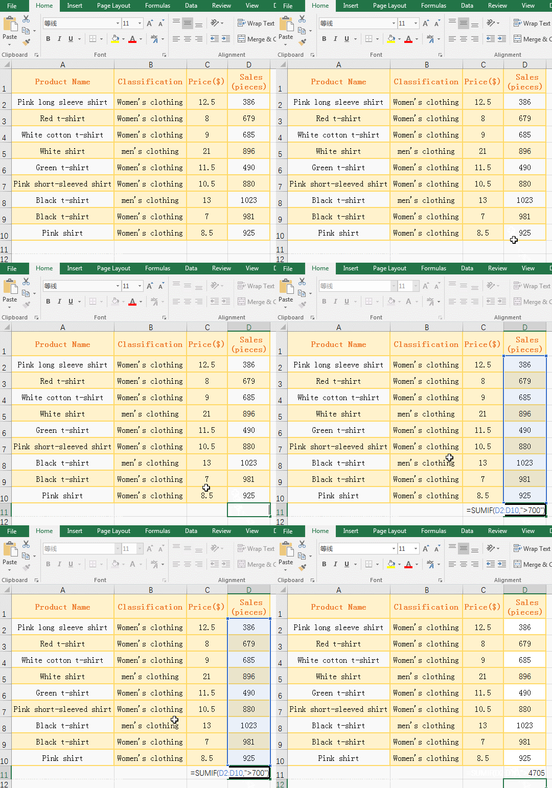
Figure 1

2. The formula =SUMIF(D2:D10,">700") omits the actual cells that are added, so the conditional area Range(D2:D10) is used as the summation range. ">700" is a condition, meaning that each value in D2 to D10 is compared with 700, and if it is greater than 700, it is included in the summation.

Hint: The condition ">700" can also be written like this: ">"&"700", To separate the greater than and numerical wrote, and then use & to connect.

(2) There are Sum_Range argument

1. If you want to sum only the values that are sales of all men's wear. Double-click the cell D11, and copy the formula =SUMIF(B2:B10, "Men's clothing", D2:D10), and paste it in cell D11, press Enter, return to the result 1919; the operation steps, as shown in Figure 2:

Figure 2

2. Formula =SUMIF(B2:B10, "Men's clothing", D2:D10), The range B2:B10 is the conditional area, the condition is "Men's Wear", the range D2:D10 is the actual summation area, meaning: If there are "men's clothing" in the range B2:B10, the corresponding value of F2:F10 is included in the summation; for example, "men's clothing" in B5, D5 is included in the summation.

(3) There are wildcards such as question marks(?) or asterisks(*) in criteria

1) With question marks(?) in criteria

1. Sum of the sales of all clothes that contain exactly six charaters + "t-shirt". Double-click the cell D11, and copy the formula =SUMIF(A2:A10,"??????t-shirt", D2:D10), and paste it in cell D11, press Enter, return to the result 2494; the operation process steps, as shown in Figure 3:

Figure 3

2. The "??????t-shirt" is criteria in formula =SUMIF(A2:A10,"??????t-shirt", D2:D10). There are six question marks in criteria. Each question mark matches a character, which means to find out all clothes from the range A2:A10, It consists of 13 charaters, the first 6 characters can be any character, and the last 7 characters must be "t-shirt".

2)  With asterisk(*) in criteria

1. Sum of the sales of all clothes that end with "t-shirt", or that begin with "Pink", or that begin with "Pink" and end with "t-shirt". Double-click the cell D11, and copy the formula =SUMIF(A2:A10,"*t-shirt", D2:D10), and paste it in cell D11, press Enter, return to the result 3858.

  Double-click the cell D11, change the criteria in the formula to "Pink*", press Enter, return  result 2191; double-click cell D11 again, change the criteria in the formula to "Pink*t-shirt", press Enter, return to the result 0; the operation steps, as shown in Figure 4:

Figure 4

2. Formula description:

A, The "*t-shirt" is criteria in the formula =SUMIF(A2:A10,"*t-shirt", D2:D10), the * in the criteria matches any character, it can be one or more; the meaning of the criteria is looking for Clothes end with "t-shirt".

B. The "Pink*" is criteria in the formula =SUMIF(A2:A10,"Pink*", D2:D10), it means finding the clothes that begin with "Pink".

C, The "Pink*t-shirt" is criteria in the formula =SUMIF(A2:A10,"Pink*t-shirt", D2:D10), it means to find out the clothes that begin with "Pink" and end with "t-shirt".

(4) With function in criteria

1. Sum of the sales of all clothes that is greater than and equal to the average sales volume of the clothes. Double-click the cell D11, and copy the formula =SUMIF(D2:D10,">="&AVERAGE(D2:D10)), and paste it in cell D11, press Enter, return to the result 4705; the operation process steps, as shown in Figure 5:

Figure 5

2. The ">="&AVERAGE(D2:D10) is criteria in the formula =SUMIF(D2:D10,">="&AVERAGE(D2:D10), and the criteria AVERAGE(D2:D10) is used for average sales of clothes.

II, Examples: The argument Sum_Range of SumIf function in Excel is different Range in size and shape

<I> Sum_Range and Range are both in a column

(I) Sum_Range is on, Range is under

1. Double-click the cell D11, copy the formula =SUMIF(B5:B10, "Men's clothing", D2:D5), paste it in cell D11, press Enter, return to the result 1282; the operation steps, as shown in Figure 6:

Figure 6

2. Formula description:

The actual summation range Sum_Range is D2:D5, the criteria Range is B5:B10, the two ranges are different in size and shape, D2:D5 is on, B5:B10 is under, B5 is corresponding to D2, and B6 is corresponding to D3, others and so on, which are equivalent that the range C5:C10 were moved to up. only C5 and C8 in C5:C10 are "men's clothing", they correspond to D2 and D5, and the sum formula is 386 + 896 = 1282.

(II) Sum_Range is under, Range is on

1. Double-click the cell D11, copy the formula =SUMIF(B2:B6, "Men's clothing", D5:D10), and paste it in cell D11, press Enter, return to the result 982, the operation steps, as shown in Figure 7:

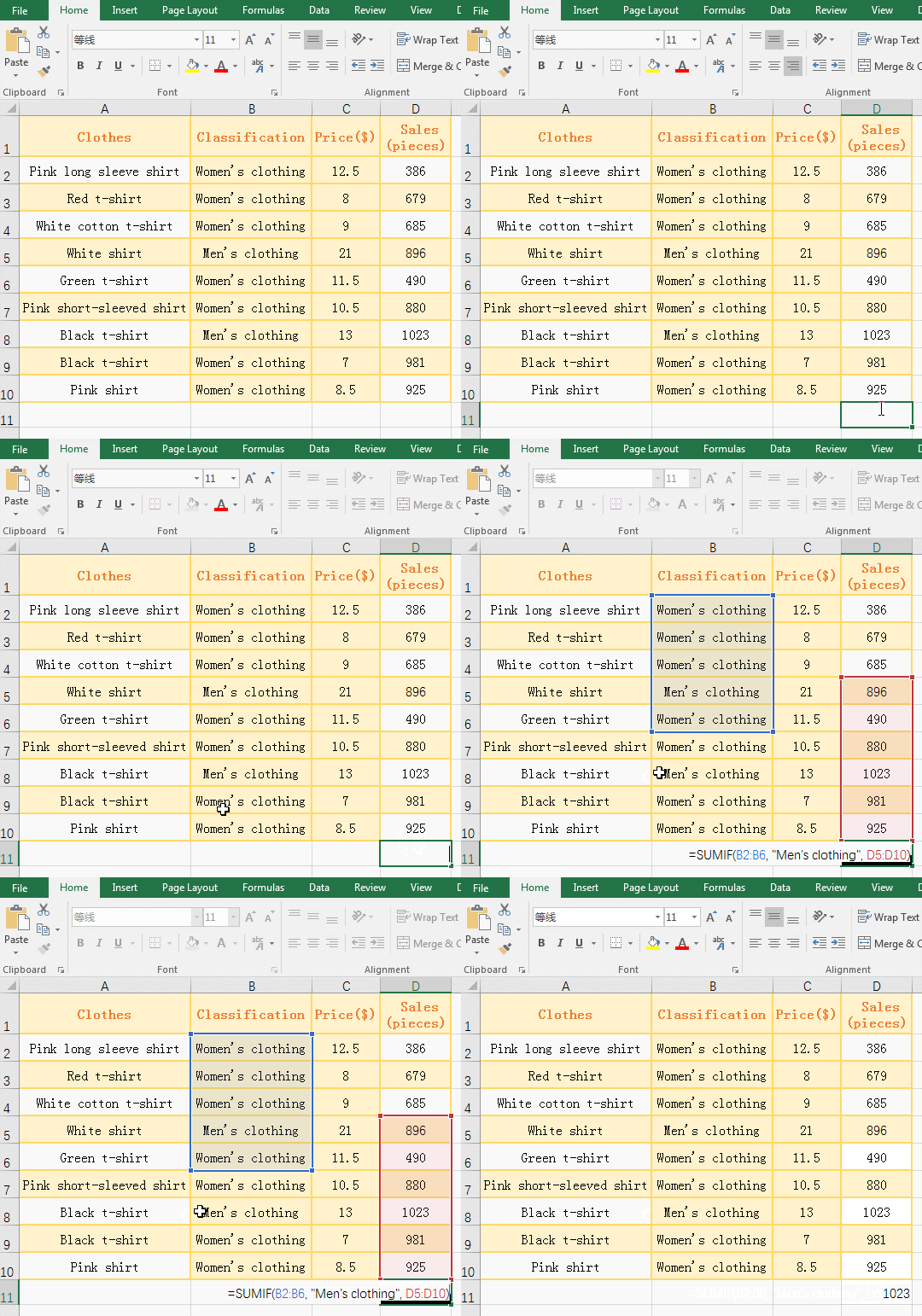
Figure 7

2. Formula description:

The actual summation range Sum_Range is D5:D10, the criteria Range is B2:B6, D5:D10 is below, B2:B6 is up, B2 is corresponding to D5, B3 is corresponding to D6, and so on, which are equivalent that the range B5:B10 were moved to down; only B5 in B2:B6 is "Men's clothing", it corresponds to D8, so it returns the value 1023 of D8.

(III) Sum_Range is the same as the starting position of Range

1. Double-click the cell D11, and copy the formula =SUMIF(B2:B6, "Men's clothing", D2:D10), and paste it in cell D11, press Enter, return to the result 896, the operation steps, as shown in Figure 8:

Figure 8

2. Formula description:

The actual summation range Sum_Range is D2:D10, and the criteria Range is B2:B6. The starting positions of the two ranges are the same, except that D2:D10 has four more cells than B2:B6, and the extra cells in the summation are ignored. However, only B5 in B2:B6 is "men's clothing", and B5 is corresponding to D5, so the value of D5 is returned to 897.

<II> Sum_Range and Range are both columns

(I) Sum_Range is on, Range is under

1. Double-click the cell E10, copy the formula =SUMIF(B5:C9,">600",D2:E6), and paste it in cell E10, press Enter, return to the result 776; the operation steps are as shown in Figure 9:

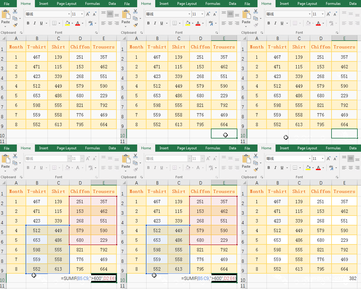
Figure 9

2. Formula description:

The actual summation range Sum_Range is D2:E6(on), and the criteria Range is B5:C9(below); their correspondence is: B5 corresponds to D2, C5 corresponds to E2, B6 corresponds to D3, and C6 corresponds to E3, and others By analogy. imilarly, B5:C9 is shifted up; only B6 and C9 are greater than 600 in B5:C9, they correspond to D3 and E6, respectively, and the sum formula is 153 + 229 = 582.

(II) Sum_Range is under, Range is on

1. Double-click the cell E10, copy the formula =SUMIF(B2:C6,">600", D4:E8), and paste it in cell E10, press Enter, return to the result 776; the operation steps are as shown in Figure 10:

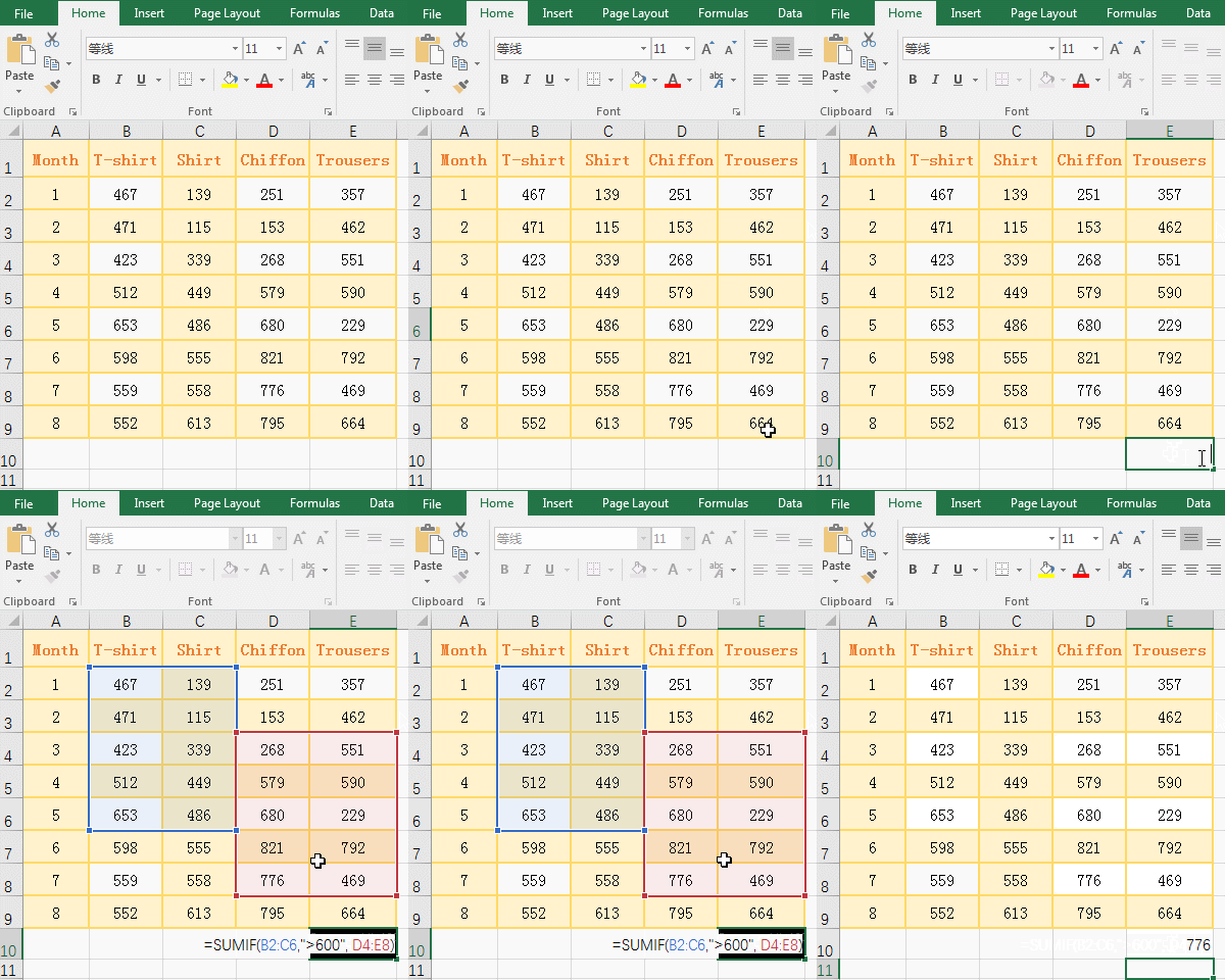
Figure 10

2. Formula description:

The actual summation range Sum_Range is D4:E8 (below), and the criteria Range is B2:C6 (on); their correspondence is: B2 corresponds to D4, C2 corresponds to E4, B3 corresponds to D5, C3 corresponds to E5, and others By analogy, it is equivalent to shifting B2:C6 downwards. in B2:C6, only B6 is greater than 600, it corresponds to D8, and the value of D8 is 776, so the sum result returns 776.

III, Excel SumIf function extension use case

(1) Excel SumIf multiple criteria(Sum + SumIf)

1. The sum of all clothing sales that art starting with "white or black". Double the cell D11, and copy the formula =SUMIF(A2:A10,{"white*","black*"},D2:D10), and paste it in cell D11, press Enter, return to the result 1581; double-click D11 to change the formula for =SUM(SUMIF(A2:A10,{"white*","black*"},D2:D10)), press Enter to return to the result 3585; the operation steps are as shown in Figure 11:

Figure 11

2. Formula description:

A. The {"white*", "black*"} are criteria in the formula =SUMIF(B2:B10, {"white*", "black*"}, F2:F10), which is an array of two elements. The criteria are used to find out the clothes that begin with white or black; but after the formula is executed, only the result that meet the first element "white*" is returned, and the result that meet the second element is gnored. if you want to meet the result of the two conditions, Excel2007 and above can use SumIfs function, Excel2007 and below can use Sum + SumIf, also demonstrate the second formula.

B. In the formula =SUM(SUMIF(A2:A10,{"white*","black*"},D2:D10)), the SumIf function is used to returned, respectively, the result that meet the two criteria {"white*","black*"}; the Sum funtion is used to added the result that is returned by SumIf function.

(2) The criteria os SumIf function with greater than and equal

1. Sum of the sales that are between 600 and 800. Double-click the cell D11, and copy the formula =SUMIF(D2:D10,">=600")-SUMIF(D2:D10,">800"), and paste in cell D11, press Enter, return to the result 1364, the operation steps, as shown in Figure 12:

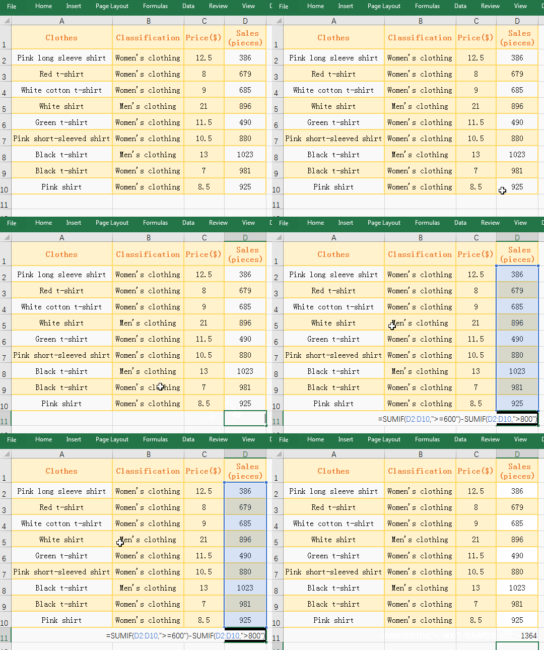
Figure 12

2. In formula =SUMIF(D2:D10,">=600")-SUMIF(D2:D10,">800"), SUMIF(D2:D10,">=600") is used to return the sum that meet criteria that is greater than an equal 600, SUMIF(D2:D10,">800") is used to return the sum that meet criteria that is greater than 800.Their difference is exactly the sum of salse that meet the criteria "D2:D10 >= 600" and "D2:D10 < 800".

IV, Syntax of Excel SumIf function

1. Expression: SUMIF(Range, Criteria, [Sum_Range])

2. Description:

A. If the Sum_Range argument is omitted, it is summed in the Range argement; if there is Sum_Range argument, it is summed in Sum_Range. If there are blank, logical, and text that cannot be converted to numbers in the summation area, they will be ignored.

B. The Criteria can be a number, any text(such as "women's clothing"), an expression (such as ">=10", "<>1"), a cell reference(such as A1), a function(such as NOW()); Text, logical, or mathematical symbols must be enclosed in double quotation marks. Numeric do not need to be enclosed in double quotes. In the condition, you can use the wildcard question mark(?) and the asterisk(*), the question mark matches a character, the asterisk matches any one or more characters; if you want to find the question mark or asterisk, use the escape character ~, for example, look up Question mark, you need to say ~?.

C, The Sum_Range argument can be different in size and shape as the Range. The actual cells that are added is taken from the cell in the upper left corner of Sum_Range to the cell in the lower right corner. Range takes the cell corresponding to Sum_Range, as shown in the example. In addition, when the Sum_Range are not the same size and shape as the Range, the execution speed is slower than the same.

D. When the string matched by the SumIf function longer than 255 characters, the value error #VALUE! will be returned.