 Office > Excel > Excel 2019 > Content
Vlookup with if statement(use if/if{0,1} combination two or three conditions)
The VLookUp function is usually used for a conditional lookup, but it can also implement multiple conditional lookups. If you combine multiple conditions, you need to use If or If{0,1}. You usually use If to find two conditions, using If{0,1}, it can achieve two conditions and can find three conditions or even more.
If you use If{0,1} to achieve more than two conditions, you need to use & to connect the search value to the search range, that is, merge the columns to satisfy the condition into one column, and then search in the column, the column that is returned is independent of one column. The following are four examples of Vlookup with if statement.
I, Vlookup if two conditions in excel
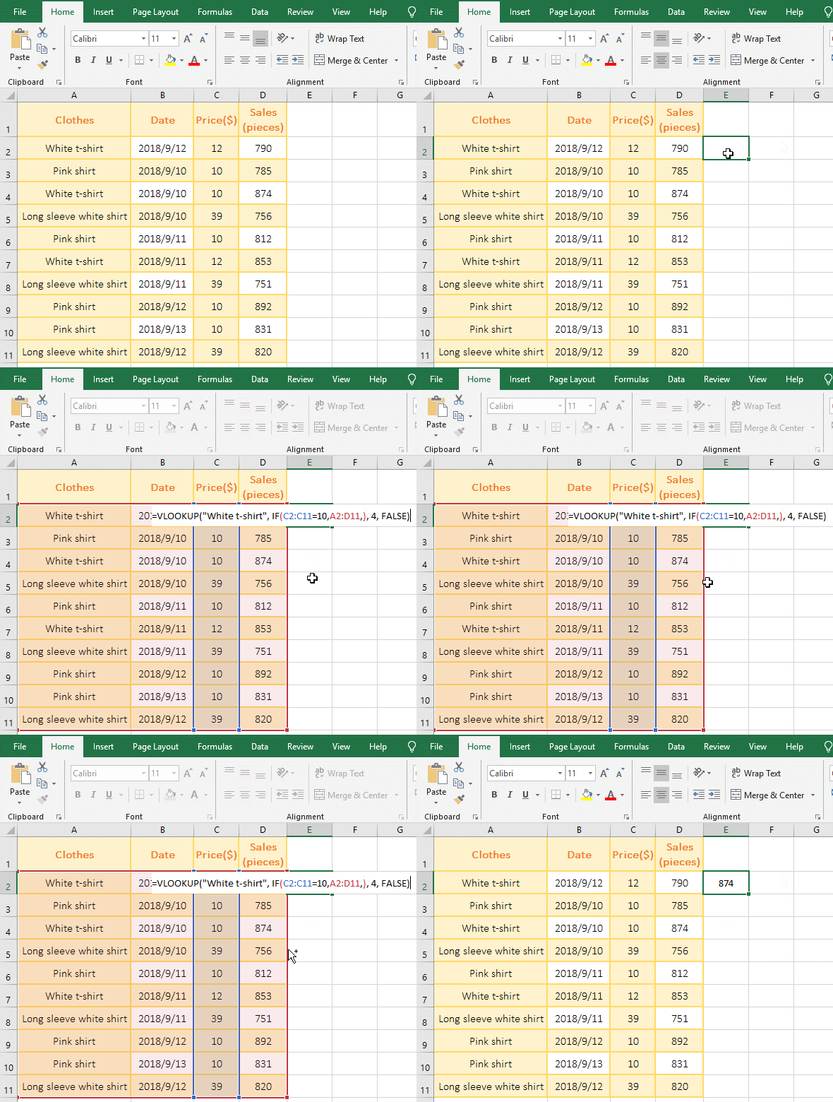
1. If you want to find "Sales" with "Clothes" as "white t-shirt" and "price" equal to 10. Double-click cell E2, copy the formula =VLOOKUP("White t-shirt", IF(C2:C11=10,A2:D11,), 4, FALSE), and paste it in E2, press Ctrl + Shift + Enter to return to the search result 874 , the operation process steps, as shown in Figure 1:

Figure 1
2, The formula =VLOOKUP("White t-shirt", IF(C2:C11=10,A2:D11,), 4, FALSE) Description:
A. C2: C11=10 is the condition of If, meaning: each value in C2 to C11 is compared with 10. If it is equal to 10, it returns True, otherwise it returns False, and finally returns the array {FALSE;TRUE;TRUE;FALSE ;TRUE;FALSE;FALSE;TRUE;TRUE;FALSE}.
B. Then IF(C2:C11=10,A2:D11,) becomes IF({FALSE;TRUE;TRUE;FALSE;TRUE;FALSE;FALSE;TRUE;TRUE;FALSE}, A2:D11,), and then each element is fetched from the array. If it is True, the data in A2:D11 is returned, otherwise it returns 0. For example: FALSE is retrieved for the first time, and "0,0,0,0;" is returned;(each 0 corresponds to one column in A2:D11); the second time to take out TRUE, return the data in A3:D3, namely ""Pink shirt",43353,10,785;", and so on. 43353 in the array is the value to which the date is converted.
C. The formula becomes =VLOOKUP("White t-shirt",{0,0,0,0;"Pink shirt",43353,10,785;"White t-shirt", 43353,10,874;......;0,0, 0,0},4,FALSE), then look up the "White t-shirt" in the array, find it and return to the 4th column, which is exactly 874; in the formula, 4 means return to the 4th column, and FALSE means "exact match".
II, Vlookup with if statement(use If{0,1} combination condition) in excel
(I) Combine a conditional to search with If{0,1}
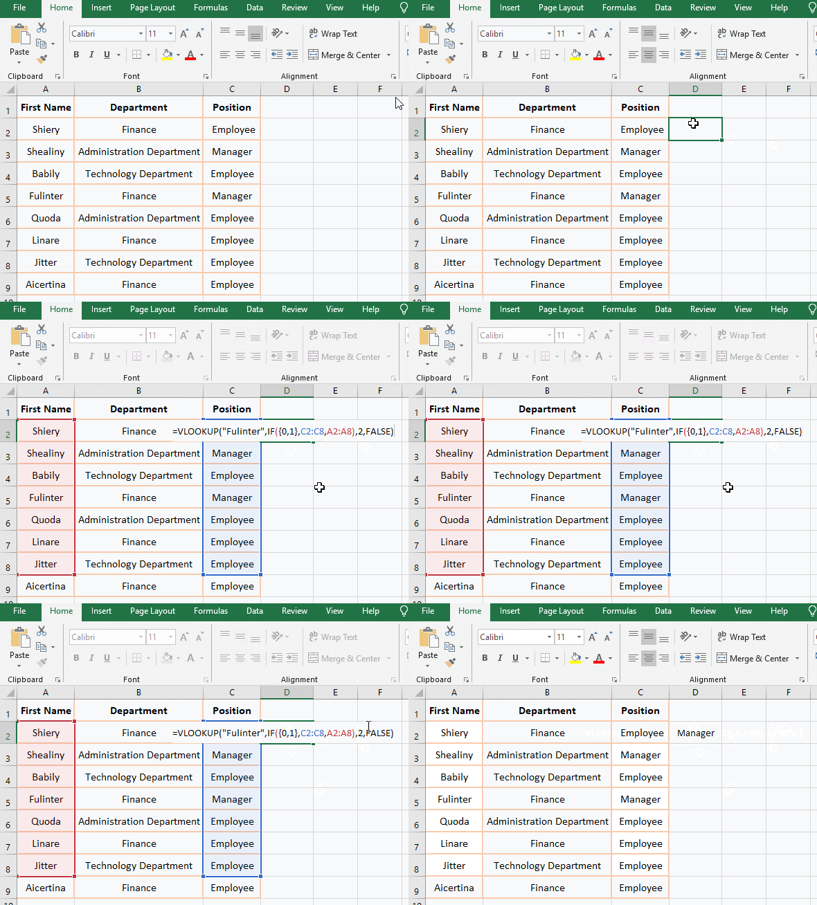
1. If you want to find the position which "First Name" is "Fulinter". Double-click cell D2, copy the formula =VLOOKUP("Fulinter",IF({0,1},C2:C8,A2:A8),2,FALSE), and paste it in D2, press Enter, return to the search result "manager"; Operation process steps, as shown in Figure 2:

Figure 2
2. Formula =VLOOKUP("Fulinter",IF({0,1},C2:C8,A2:A8),2,FALSE) explanation:
A. {0,1} are array conditions of If, IF({0,1},C2:C8,A2:A8) means: 0 is taken from the array for the first time, and 0 is False, so A2(Shiery) in A2:A9 is returned; take 1 from the array for the second time, since 1 is True, return C2(employee) in C2:C9. Then take 0 from the array again, return A3(Shealiny) in A2:A9, then take out 1 and return to C3(employee) in C3:C9; others and so on until C9 and A9 are obtained, and finally return array {"Shiery","Employee";"Shealiny","Manager";"Babily","Employee";"Fulinter", "Manager";"Quoda","Employee";"Linare","Employee";"Jitter", "Employee";"Aicertina", "Employee"}.
B. The formula becomes =VLOOKUP ("Fulinter", {"Shiery","Employee";"Shealiny","Manager";"Babily","Employee";"Fulinter", "Manager";"Quoda","Employee";"Linare","Employee";"Jitter", "Employee";"Aicertina", "Employee"}, 2, FALSE), then look for "Fulinter" in the array, return to the second column after finding in the third row, that is, return "Manager".
Hint: The array {0,1} can swap positions. If it is changed to {1,0}, the formula becomes =VLOOKUP("Fulinter",IF({1,0},A2:A9,C2:C9), 2, FALSE), A2:A9 and C2:C9 in if statement also need to exchange positions.
(II) Use If{0,1} to combine two conditions to find
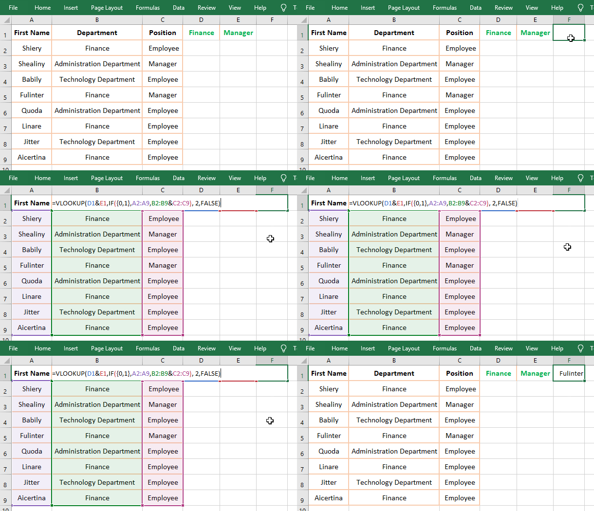
1. If you want to find the "manager" of the "Sales Department". Double-click cell F1, copy the formula =VLOOKUP(D1&E1,IF({0,1},A2:A9,B2:B9&C2:C9), 2,FALSE), paste it in F1, press Ctrl + Shift + Enter to return to the search result "Fulinter"; the process steps, as shown in Figure 3:

Figure 3
2. Formula =VLOOKUP(D1&E1,IF({0,1},A2:A9,B2:B9&C2:C9), 2,FALSE) Explanation:
A. D1&E1 connect the values ??in D1 and E1 together to form the search value "FinanceManager"; B2:B9&C2:C9 connect the data in B2 to B9 and C2 to C9 by row, for example: first time, B2 is connected with C2, which is "FinanceEmployee"; the second time, B3 is connected with C3, that is, "Administration DepartmentManager"; the others are deduced until B9 and C9 are taken; finally, the array is returned {"FinanceEmployee"; "Administration DepartmentManager"; "Technology DepartmentEmployee"; "FinanceManager"; "Administration DepartmentEmployee"; "FinanceEmployee"; "Technology DepartmentEmployee";"FinanceEmployee"}.
B. IF({0,1}, A2:A9, B2:B9&C2:C9) and IF({0,1}, C2:C9,A2:A9) that was described above is a meaning, and the result that was returned is {"FinanceEmployee", "Shiery"; "Administration DepartmentManager", "Shealiny"; "Technology DepartmentEmployee", "Babily"; "FinanceManager", "Fulinter"; "Administration DepartmentEmployee", "Quoda"; "FinanceEmployee", "Linare"; "Technology DepartmentEmployee", "Jitter"; "FinanceEmployee","Aicertina"}.
C. The formula becomes =VLOOKUP("FinanceManager",{"FinanceEmployee", "Shiery"; "Administration DepartmentManager", "Shealiny"; "Technology DepartmentEmployee", "Babily"; "FinanceManager", "Fulinter"; "Administration DepartmentEmployee", "Quoda"; "FinanceEmployee", "Linare"; "Technology DepartmentEmployee", "Jitter"; "FinanceEmployee","Aicertina"}, 2,FALSE), then look for "FinanceManager" in the array, found in the fourth row, returns to the second column, which happens to be "Fulinter".
(III) Using If{0,1} to combine three conditions to find
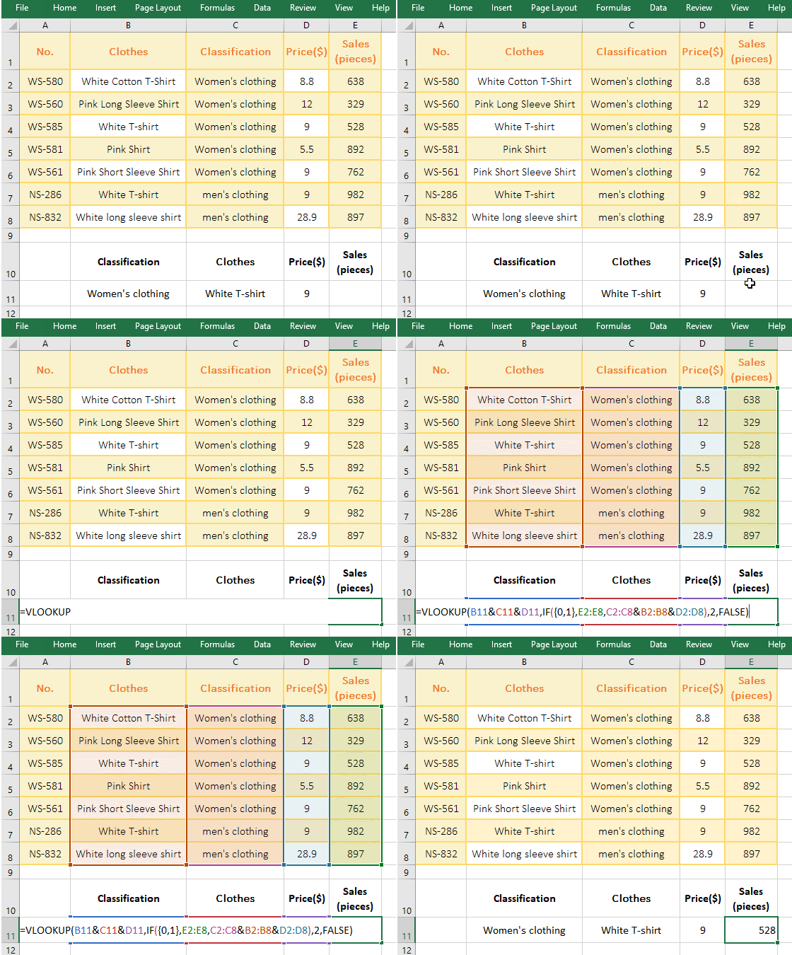
1. If you want to find the clothing sales with "Classification" as "Women's clothing", "Clothes" as "White T-Shirt" and "Price" equal to 9. Double-click the E11 cell, copy the formula =VLOOKUP(B11&C11&D11,IF({0,1},E2:E8,C2:C8&B2:B8&D2:D8),2,FALSE), and paste it in E11, press Enter, return to the search result 528; Operation process steps, as shown in Figure 4:

Figure 4
2. The meaning of formula =VLOOKUP(B11&C11&D11,IF({0,1},E2:E8,C2:C8&B2:B8&D2:D8),2,FALSE) is as with "Finding two conditions with If{0,1}". Here we just connect the three conditions into a lookup value and join the three columns into a column of lookup arrays.
Tip: Generally, the multi-condition search usually uses the LookUp function. On the one hand, it is easy to combine conditions, on the other hand, the execution speed is faster than the VlookUp function. The related content will be introduced in the following chapters.
-
Related Reading
- How to set Header and footer in word(13 examples), i
- How to start page numbers on page 3 and each section
- VLookUp in excel introduces step by step(10 examples
- Excel If function examples, include if statement nes
- How to find duplicate values in excel using vlookup(
- Excel SumIf function with ?/*, Average and array mul
- The use instances of Excel Round function, include R
- How to sort in excel(11 examples), include sort by c
- How to wrap text in excel and displays paragraph in
- How to sum in excel(9 formulas), include sum use sho
- How to create drop down list in excel and update/del