How to create drop down list in excel and update/delete, include multiple dependent(cascading)

Some spreadsheets require a drop down list if they are required to select a category, department or region. You can make a drop down list, or a dependent(cascading) drop down list, or multiple dependent drop down lists in Excel. To make them, you need to select "List" or define a name for the category. How to create drop down list in excel? The article will use three concrete examples to demonstrate the production method.

After the Excel drop down list is created, if the data source is updated, the changes will not be automatically reflected in the drop down list, and the name needs to be re-defined to update to the drop down list. Also, if you want to delete the drop down list, you need to change the "List" to "Any value".

I, How to create drop down list in excel

1. If you want to create a department drop down list. Select the C2 cell, select the "Data" tab, click "Data Varidation" icon, open the "Data Varidation" window, select the "Settings" tab, and click the drop-down list box under "Allow", select "List" from the pop-up options; click the input box under "Source" to position the cursor there, select the prepared items (ie the department in column D), click "OK"; The drop down list icon appears to the right of "Department", the drop down list is completed; the operation process steps are as shown in Figure 1:

Figure 1

2. Tip: Open the "Data Varidation" window can use the shortcut key Alt + A + V + V, the method is: hold down Alt, press A once, press V twice. In addition, if you can't select the cursor after entering the input box under "Source", just click the "arrow" icon to the right of the input box, which usually occurs in the lower version of Excel.

II, How to add drop down list in excel(Excel dependent drop down list)

If you have a fruit and vegetable table, ask for a drop down list for its "Classification 1" and "Classification 2" to facilitate the selection of the category. Since there are two categories, you need to make a dependent drop down list; you should prepare their items before making the production, in order to take data at the time of production, the following are specific production steps:

1. Create names for "Classification 1" and "Classification 2". Switch to the sheet "category", select the Vegetable and Fruit categories, select the "Formula" tab, and click "Create from selection" (or press the shortcut key Ctrl + Shift + F3) ), open the "Create names from Selection" window, only check the "Top row" (that is, the "Classification 1"), click "OK."Operation process steps, as shown in Figure 2:

Figure 2

2. Add reference data for "Classification 1". Switch to the sheet "fruit & vegetable", select cell B2, select "Data" tab, click "Data Validation" icon, open the "Data Validation" window, select the "Settings" tab, and click the drop down list under Allow, select "List"; position the cursor in the input box under "Source", switch to the sheet "category", select "Classification 1" (ie " Vegetable and Fruit"), and click "OK".

3. Add reference data to the "Classification 2". Select C2, click "Data Validation" icon, open the "Data Verification" window again, also select the "Settings" tab, "Allow" also select "List", put formulas =Indirect($B2) Copy to the input box of "Source" and click "OK".

4. Extend the created dependent drop down list to each row with data. Select B2:C2, move the mouse to the cell fill handle on the lower right corner of C2, after the mouse turns into a bold black cross, hold down the left button, drag down until the last row, then the B3:C8 create dependent drop down lists. Clicking on the first and second drop down lists, they have the corresponding options. Operation process steps, as shown in Figure 3:

Figure 3

The formula =Indirect($B2) indicates that the C2 references the B2, that is, the "Classification 2" references the "Classification 1"; the $B2 represents the absolute reference to the column, and the relative reference to the row, that is, when the row is dragged down, the column does not change, such as B2 Will become B3, B4, ....

III, How to create drop down list in excel(Multiple dependent(cascading) drop down list)

For example, to change the dependent drop down list created above to the multiple dependent drop down list. You must also prepare the items for drop down lists in advance. Since the "Classification 2" include multiple items, only select two categories(ie  Cruciferae and Simple Fruit) here. The following is to make steps.

1. Create a name for the "Classification 3". The current sheet is "category", select D1:E4, select the "Formula" tab, click "Create from selection", open "Create Names from Selection" window, only check the "Top row" (that is, only check "Classification 2"), click "OK".

2. Add reference data for the "Classification 3". Switch to the sheet "fruit & vegetable", select D2, select the "Data" tab, click "Data Validation" icon, open the window, select the "Settings" tab, "Allow" select "List", put the formula =INDIRECT(Substitute($C2," ","_")) Copy to under "Source", let D2 reference C2, click "OK".

3. Extend the created third drop down list to all rows with data. Move the mouse to the cell fill handle on the lower right corner of D2. After the mouse changes to the bold black cross, hold down the left button and drag down until the last row. The cells that pass through have a drop down list. When you click them, there are already options that dependent "Classification 2"; the operational steps are shown in Figure 4:

Figure 4

4. The formula =INDIRECT(Substitute($C2," ","_")) description

If there are spaces in the definition name, excel will automatically replace the space with "_", and the name of the "Fruit" class has spaces, so when you reference C2 in D2, you need to replace the space with "_", which is expressed as Substitute. ($C2," ","_") to ensure that the definition name matches the name in the cell (such as B2), as shown in Figure 5:

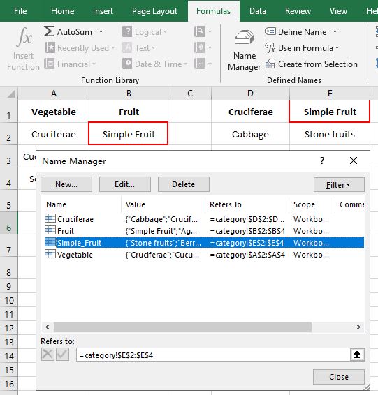
Figure 5

IV, If the second or third classification include empty cells, how to select?

Since the items of each category are not necessarily the same, there will be cases where there are empty cells, and the options of  drop down list does not allow null values in excel, so the empty cells cannot be selected, and the above operation method have selected the empty cells. so for this case to use the "Special" to choose, as follows:

Select the category that include empty cells, such as D1:E5, press Ctrl + G, open the "Go To" window, click "Special", select "constants" in the window that opens, click "OK" to select only the cells with data, the process steps, as shown in Figure 6:

Figure 6

V, Excel drop down list how to update the data source after modification

1. "Citrus" was added as a new item of "Simple Fruit" in the previous step (IV, If the second or third classification include empty cells, how to select?), it will not Automatically update to the drop down list, you need to define the name for the "Simple Fruit" again, the operation process steps, as shown in Figure 7:

Figure 7

2. The operation step description: D1:D4 and E1:E5 have selected in the previous step, select the "Formula" tab, click "Create from Selection", open the "Create Names from Selection" window, click "OK" in the pop-up window, then new item of "Simple Fruit" is  updated go to the drop down list, expand the drop down list that dependent "Simple Fruit" to have "Citrus" option.

VI, Excel drop down list delete method

Select the cell to delete the drop down list(e.g D2:D9), hold down Alt, press A once, press V twice, open the "Data Validation" window, "Allow" to select "Any value", click "OK", then the drop down lists in D2:D9 are deleted, and the operation steps are as shown in Figure 8:

Figure 8

Tip: If you want to delete the contents of cells and the drop down list at the same time, after selecting the cells, you can hold down Alt and press E and A respectively.