Excel SumProduct function(multiple criteria, with if and text, combine conditions with * and +)

The SumProduct function can be used for both sum and sum of product in excel. It is divided into an array and a multi-condition expression, the array expression is used to calculate the sum of product, up to 255 arrays; the conditional expression is used to calculate the sum of the specified conditions, it is divided into two forms, one is separated by a comma and there must be -- before the condition, and the other is that the Sum_Range and condition are connected by an asterisk(*), regardless of Which condition form, the relationship between the conditions is "AND".

In addition to the asterisk(*) for the "AND" relationship, the SumProduct function can also use the plus sign(+) to indicate the  "OR" relationship. Usually several conditions are joined with a plus sign in a formula to indicates "OR" relationship.

I, Excel SumProduct function syntax

1. Array expression: SUMPRODUCT(Array1, [Array2], [Array3], ...)

Description: SumProduct function must have at least one array, at most 255 arrays; if there are more than two arrays, the array must have the same dimension, otherwise it will return the value error #VALUE!; non-numeric type is treated as 0; Each array must have the same dimension; it is calculated by multiplying the corresponding elements of each array and summing them.

2. Conditional expression: SUMPRODUCT (Sum_Range, --(Criteria 1), [--(Criteria 2),...])

Or SUMPRODUCT((Sum_Range)*(Criteria 1)*[(Criteria 2),...])

Note: Enclosed in [] in the conditional expression is optional, that is, the SumProduct function must have at least one Criteria; if there are more than two Criteria, the Criteria are "AND" relationship, that is, multiple Criteria must be met at the same time. The order of the Sum_Range and Criteria can be exchanged; the -- in front of the Criteria is to convert the logical value or the null value into a number for calculation, and the asterisk(*) represents the "AND" relationship.

II, Excel SumProduct function array expression examples

(I) An instance with two arrays

1. If Adds the total turnover of clothes Sales. Select cell E9, copy the formula =SUMPRODUCT(D2:D8,E2:E8), and paste it in E9, press Enter, return to 60734.1; the operation steps are as shown in Figure 1:

Figure 1

2. The formula refers to two cell regions(array), namely D2:D8 and E2:E8. The calculation method is: D2 * E2 + D3 * E3 + ... + D8 * E8.

Hint: If you only sum and write only one array, for example, sum the clothing sales =SUMPRODUCT(E2:E8).

(II) Non-numeric type is treated as 0

1. Select the cell B1, copy the formula =SUMPRODUCT(A1:A5) to B1, press Enter, return to 3; the operation steps are as shown in Figure 2:

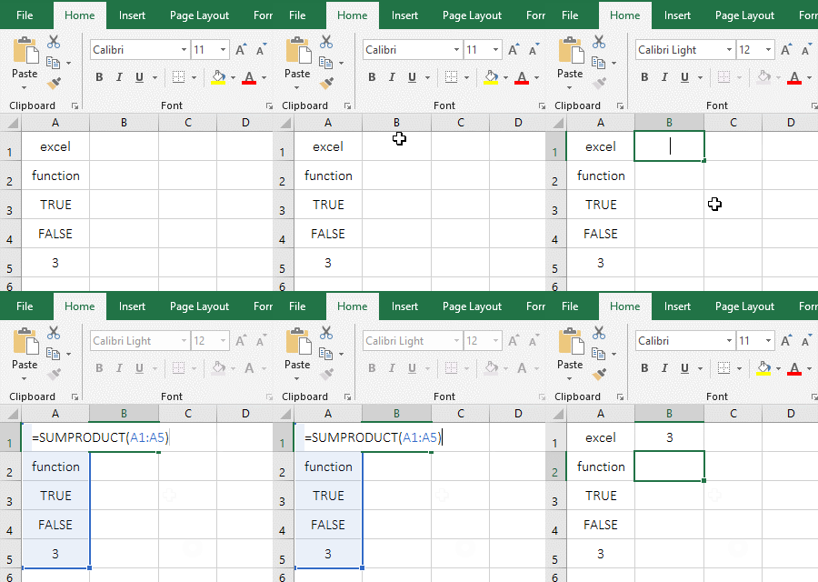
Figure 2

2. There is only one number 3 in A1:A5, and the return result is 3, indicating that the non-numeric type is ignored, and the logical value True does not change to 1.

(III) An instance of the return value error #VALUE!

1. Select the cell C1, copy the formula =SUMPRODUCT(A1:A5,B2:B5) to C1, press Enter, return the value error #VALUE!; The operation steps are as shown in Figure 3:

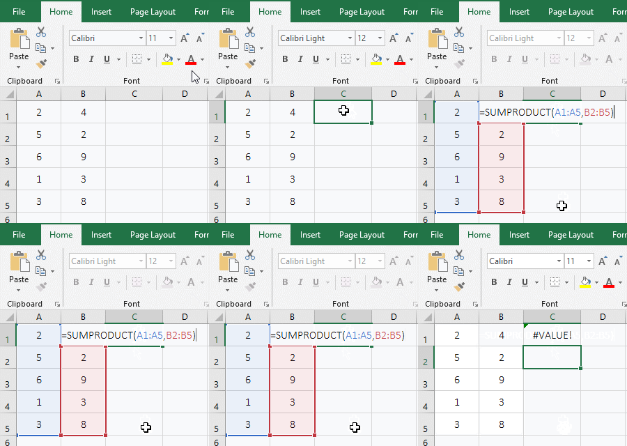
Figure 3

2. In the formula, A1:A5 has one more cell than B2:B5, that is, the array dimension is different, so the return value is wrong #VALUE!.

III, Excel sumproduct multiple criteria expression examples

(1) SUMPRODUCT(Sum_Range, --(Criteria 1), [--(Criteria 2),...])

1. If add the "Sales" of Clothes whose "Classification" equal "Women's clothing" and the "price" is greater than 8. Select the cell E9, copy the formula =SUMPRODUCT(E2:E8,--(C2:C8="Women's clothing"),--(D2:D8>8)) to E9, press Enter, return to the summation result 2257; Operation process steps, as shown in Figure 4:

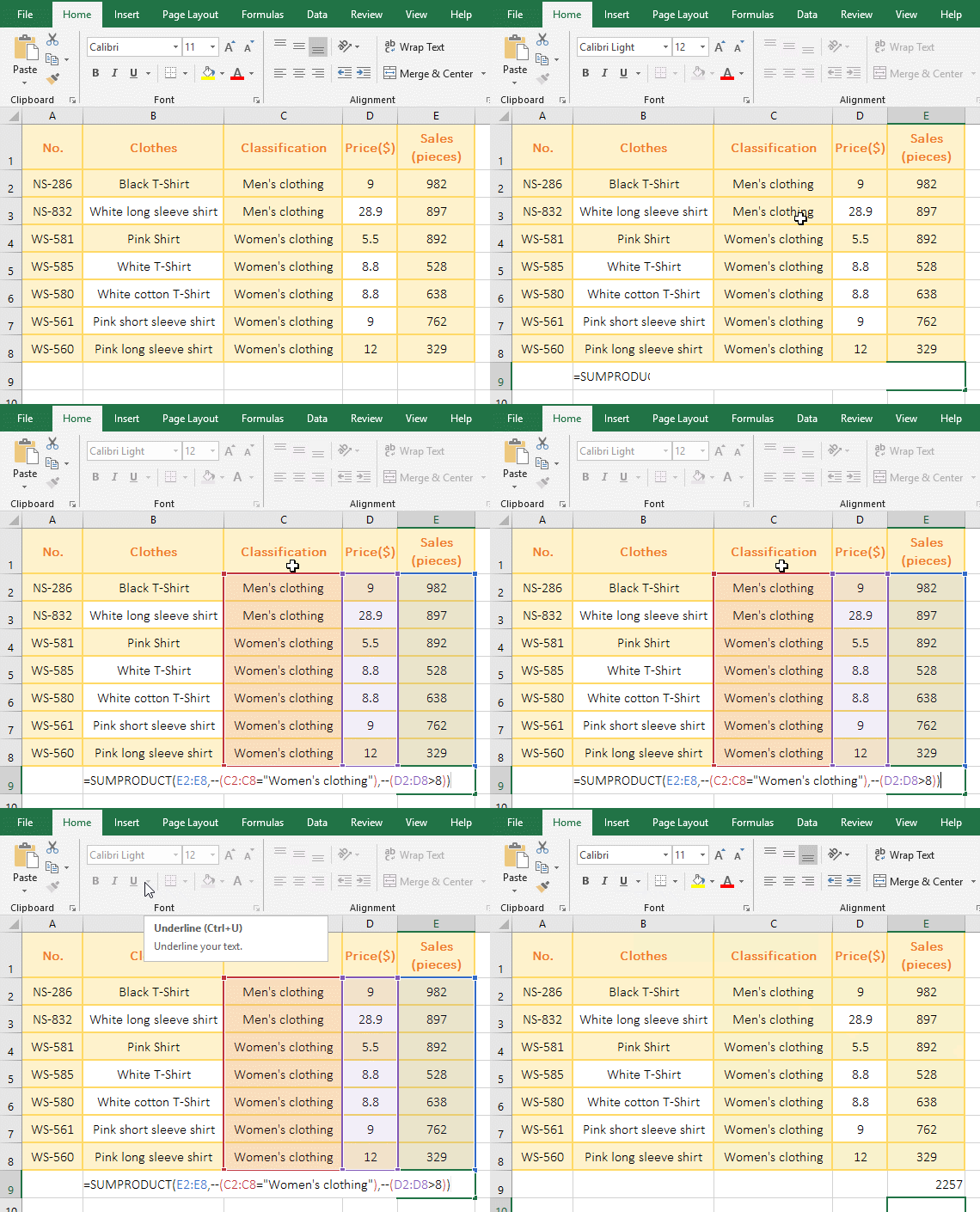
Figure 4

2. Formula =SUMPRODUCT(E2:E8,--(C2:C8="Women's clothing"),--(D2:D8>8)) description(Sumproduct with text):

A. The Sum_Range of the formula is E2:E8, the Criteria are --(C2:C8="Women's clothing"),--(D2:D8>8); the first Criteria --(C2:C8="Women's clothing") is used to take each "Classification" from C2 to C10 in turn, and compare it with "Women's clothing"; if they equal, returns to True, otherwise return False; finally returns array {FALSE;FALSE;TRUE;TRUE;TRUE;TRUE;TRUE}.

B. The second Criteria --(D2:D8>8) is used to take each price from D2 to D8 and compare it with 8; If it is greater than 8, it returns True, otherwise it returns False; finally returns the array {TRUE;TRUE;FALSE;TRUE;TRUE;TRUE;TRUE}.

C. Then two Criteria --(C2:C8="Women's clothing"),--(D2:D8>8) becomes --({FALSE;FALSE;TRUE;TRUE;TRUE;TRUE;TRUE}),--{TRUE;TRUE;FALSE;TRUE;TRUE;TRUE;TRUE}), further calculation converts True to 1, and False to 0, ie {0;0;1;1;1;1;1},{1;1;0;1;1;1;1}, and then multiply the corresponding elements of the two arrays, the result is {0;0;0;1;1;1;1}.

D. E2:E8 returns an array {982;897;892;528;638;762;329}, then the formula becomes =SUMPRODUCT({982;897;892;528;638;762;329}, {0;0;0;1;1;1;1}), then multiply the corresponding elements of the two arrays and add their results, so the summation result is 2257.

(2) SUMPRODUCT((Sum_Range)* (Criteria 1)*[(Criteria 2),...])

1. The above cases, for example. Select the F11 cell, copy the formula =SUMPRODUCT((E2:E8)*(C2:C8="Women's clothing")*(D2:D8>8)) to E10, press Enter, return to the summation result 2257; The steps are as shown in Figure 5:

Figure 5

2. Formula description:

Formula =SUMPRODUCT((E2:E8)*(C2:C8="Women's clothing")*(D2:D8>8)) is another way of writing of the formula in the above example =SUMPRODUCT(E2:E8,--(C2:C8="Women's clothing"),--(D2:D8>8)), is that it connects the three parameters with * to indicate the "AND" relationship.

IV, Excel SumProduct function extension case

(I) Combine the Criteria of "AND" and "OR" with * and +(Excel sumproduct multiple criteria)

1. If adds the "Sales" of Clothes whose "Classification 1" equal "Women's clothing" and whose Classification 2" equal "Shirt or T-Shirt". Select cell F9, copy the formula =SUMPRODUCT((F2:F8)*(C2:C8="Women's clothing")*((D2:D8="Shirt")+(D2:D8="T-Shirt"))) to F9, press Enter, return to the summation result 3149; the operation steps, as shown in Figure 6:

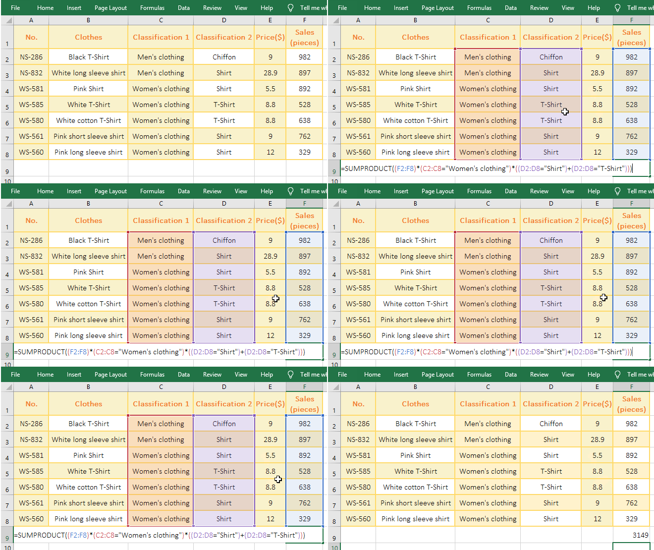
Figure 6

2. Formula =SUMPRODUCT((F2:F8)*(C2:C8="Women's clothing")*((D2:D8="Shirt")+(D2:D8="T-Shirt"))) description(Sumproduct with text):

The Criteria of the formula is (C2:C8="Women's clothing")*((D2:D8="Shirt")+(D2:D8="T-Shirt")), the former Criteria and the last two Criteria are "AND" relationship , connected by *; the latter two conditions are "OR" relationship, with + connection; meaning to select the  Clothes Sales when C2:C8 for "Women's clothing" and D2:D8 for "Shirt" or "T-Shirt".

(II) SumProduct function Sum_Range has text processing method(Sumproduct if, Sumproduct with text)

1. If adds the "Sales" of Clothes whose "Classification 1" equal "Women's clothing" and whose Classification 2" equal "Shirt", there are text in "Sales" column. Select cell F9, copy the formula =SUMPRODUCT(IF(ISTEXT(F2:F8),0,F2:F8)*(C2:C8="Women's clothing")*(D2:D8="Shirt")) to F9. Press Ctrl + Shift + Enter to return to the summation result 1983, the operation steps, as shown in Figure 7:

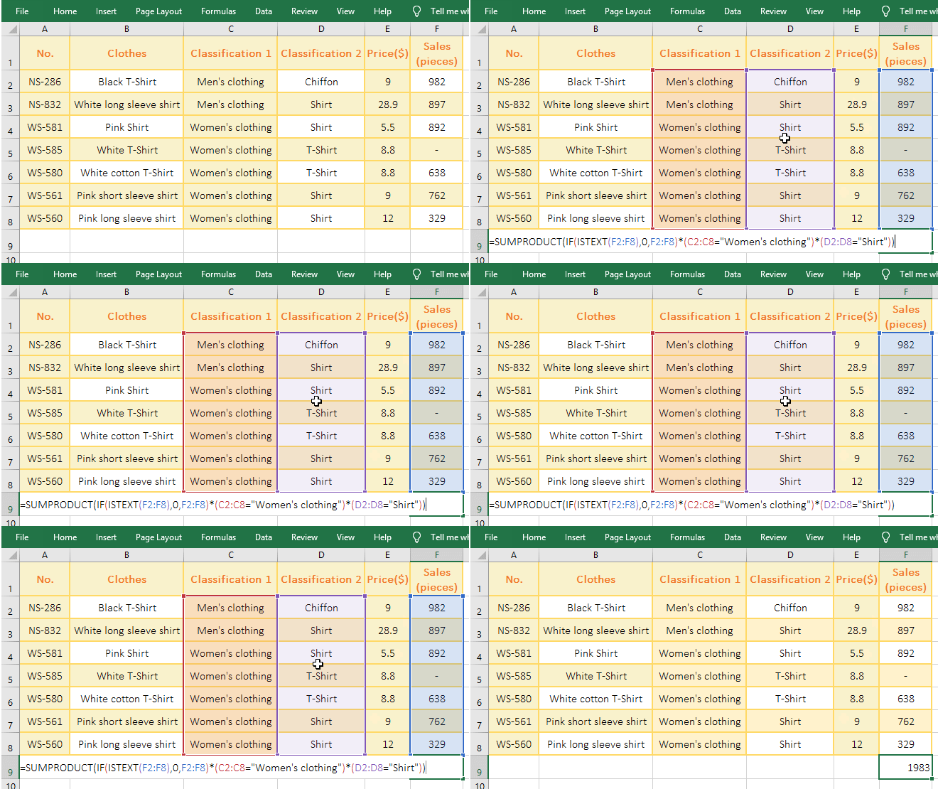
Figure 7

2. Formula =SUMPRODUCT(IF(ISTEXT(F2:F8),0,F2:F8)*(C2:C8="Women's clothing")*(D2:D8="Shirt")) description:

A. The IF(ISTEXT(F2:F8),0,F2:F8) in the formula is the Sum_Range. Since there is text(-) in the Sum_Range F2:F8, if F2:F10 is written directly, the value #VALUE! will be returned incorrectly, so use If to judge.

B. ISTEXT(F2:F8) is used to determine whether each element in F2:F8 is text. If it is text, it returns True, otherwise it returns False. Since only F5 is text, it returns the array {FALSE;FALSE;FALSE;TRUE;FALSE;FALSE;FALSE},

C. Then each element is taken out of the array in turn, if it is true, it returns 0, otherwise it returns the corresponding value in F2:F10. For example, the first time takes the first element FALSE from the array, returns 982, the second takes the second element FALSE from  the array, returns 897, and so on, and finally returns the array {982;897;892;0;638;762;329}.

3. The above formula can also be changed to =SUM(IF(ISTEXT(F2:F8),0,F2:F8)*(C2:C8="Women's clothing")*(D2:D8="Shirt")), also to press Ctrl + Shift + Enter.