Sumifs example step by step in excel(sumifs with text criteria, array and date condition)

The SumIfs function is used to sum multiple conditions in excel. The difference from the SumIf function is that SumIfs can combine multiple conditions, and SumIf can only combine one condition. The SumIfs function must have at least one Criteria_Range/Criteria pair and at most 127 Criteria_Range/Criteria pairs.

If you want to use the SumIfs function to sum with multiple conditions in the same column, if the condition is an AND relationship, you can combine two  Criteria_Range/Criteria pairs; if the condition is an OR relationship, you can combine multiple conditions with an array.  For example, if the sum within the specified date is required, that is, the condition is "AND", the former is used; if the sum of several categories is required, that is, the condition is "OR", the latter is used.

I, Excel SumIfs function syntax

1. Expression: SUMIFS(Sum_Range, Criteria_Range1, Criteria1, [Criteria_Range2, Criteria2], ...)

2. Description:

A. SumIfs function must have at least three parameters(ie Sum_Range, Criteria_Range1, Criteria1), the latter two parameters are Criteria_Range and Criteria, that is,  Criteria are set in the Criteria_Range; Criteria_Range1 and Criteria1 form a Criteria_Range1/Criteria1 pair. The SumIfs function must have at least 1 Criteria_Range/Criteria pair and at most 127 Criteria_Range/Criteria pairs.

B. If there are null values, logical values(True or False), and text that cannot be converted to numbers in Sum_Range, they are ignored.

C. There can be numbers, characters(such as "women's clothing"), expressions(such as ">= 0", "<>1"), cell references(A1), functions(such as NOW()) in the Criteria. Text, logical values, or mathematical symbols must be enclosed in double quotes in the Criteria. Individual numbers do not need to be enclosed in double quotes. You can use the wildcard question mark (?) and the asterisk(*) in the Criteria, the question mark represents a character, the asterisk indicates any one or more characters; if you want to find the question mark or asterisk, use the escape character ~, for example, look up Question mark, you need to say ~?.

D. Sum_Range and Criteria_Range must be the same size, ie they must have the same number of rows and columns, which is different from the SumIf function.

II, Sumifs example step by step in excel(Sumifs with text criteria)

(I) There is only one Criteria_Range/Criteria pair (The Sum_Range is the same column as the Criteria_Range)

1. If adds the "Sales" of clothes whose "Classification" equal "Men's clothing" or whose sales exceeds 800. Select cell E9, copy the formula =SUMIFS(E2:E8,C2:C8,"Men's clothing") to E9, press Enter, return to the summation result 1879; double-click E9 and change the formula to =SUMIFS(E2:E8,E2:E8,">800"), press Enter, return to the summation result 2771; the operation process steps, as shown in Figure 1:

Figure 1

2. E2:E8 is the Sum_Range, C2:C10 is the Criteria_Range, and "Men's clothing" is the Criteria in the formula =SUMIFS(E2:E8,C2:C8,"Men's clothing"), meaning that adds the sales of clothing that equal "Men's clothing" in C2:C8, that is, adds the E2 and E3 that correspond to C2 and C3.

3. The Sum_Range and Criteria_Range are both F2:F10 and the Criteria is ">800" in the formula =SUMIFS(E2:E8,E2:E8,">800") , that is, the sum of all clothing sales with the sales greater than 800.

(II) There are two Criteria_Range/Criteria pairs

1. If adds the "Sales" of clothes whose "Classification" equal "Women's clothing" and whose price is greater than or equal to 9. Select  cell E9 and copy the formula =SUMIFS(E2:E8,C2:C8, "Women's clothing", D2:D8,">=9") to E9, press Enter, return to the summation result 1091; as shown in Figure 2:

Figure 2

2. Formula =SUMIFS(E2:E8,C2:C8, "Women's clothing", D2:D8,">=9"), the first Criteria_Range/Criteria pair is "C2:C8,"Women's clothing"", ie Find all garments that are "Women's clothing" in C2:C8; the second Criteria_Range/Criteria pair is "D2:D8,">=9"", that is, find all garments with price greater than or equal to 9 in D2:D8; two conditions are the "AND" relationship, that is, to find all the clothing sales that are both women's clothing and the price is greater than or equal to 9, and then sum them.

(III) There are wildcards question marks(?) or asterisks(*) in Criteria

(1) Criteria with question mark(?)

1. If adds the "Sales" of Clothes that are start with "Pink" and there are only six characters after "Pink". Select cell E9, copy the formula =SUMIFS(E2:E8, B2:B8, "Pink??????") to E9, press Enter, return to the summation result 892; the operation steps, as shown in Figure 3:

Figure 3

2. The Criteria_Range in formula =SUMIFS(E2:E8, B2:B8, "Pink??????") is B2:B8, the Criteria is "Pink??????", the Criteria means that start with "Pink" and there are only six characters after "Pink"; there are three cells starting with "Pink" in B2:B10, which are B2, B7 and B8, respectively, and only "Pink" in B4 has only six characters, so the summation result is the value in F10 that correspond to B4.

(2) Criteria with asterisk (*)

1. If adds the "Sales" of Clothes that start with "White" and end with "shirt". Select the F11 cell and copy the formula =SUMIFS(E2:E8,B2:B8,"White*",B2:B8,"*shirt") to E9, press Enter, return to the summation result 2063; operation steps, As shown in Figure 4:

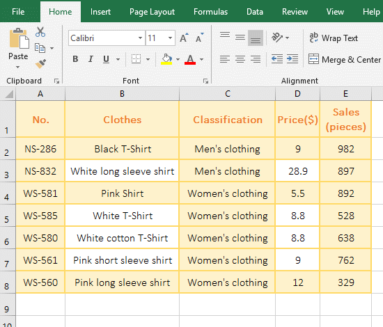
Figure 4

2. Formula description:

A. "B2:B8,"White*"" is the first Criteria_Range/Criteria pair of the formula =SUMIFS(E2:E8,B2:B8,"White*",B2:B8,"*shirt"), meaning find the Clothes that starts with "White" in B2:B10, and the * in the Criteria means any one or more characters.

B. "B2:B8,"*shirt"" is the second Criteria_Range/Criteria pair of the formula =SUMIFS(E2:E8,B2:B8,"White*",B2:B8,"*shirt"), meaning find the clothes in B2:B8 that starts with any one or more characters and ends with "shirt."

(IV) Examples of Criteria with function

1. If adds the "Sales" of Clothes whose "Classification" equal "Women's clothing" and whose "Sales" is greater than or equal to the average Sales. Select cell E9 and copy the formula =SUMIFS(E2:E8,C2:C8, "Women's clothing", E2:E8,">"&AVERAGE(E2:E8)) to E9, press Enter, return to the summation result 1654; Operation process steps, as shown in Figure 5:

Figure 5

2. The formula first Criteria_Range/Criteria pair "C2:C8,"Women's clothing"" is to find all "Women's clothing" in C2:C8; the second Criteria_Range/Criteria pair is "E2:E8,">"&AVERAGE(E2:E8)" that means to find out the clothing that is larger than the average Sales of all clothing in E2:E8. AVERAGE(E2:E8) is used to return the average Sales of all clothing.

III, Excel SumIfs function extension use case

(I) The SumIfs function uses an array to combine the same column and multi-conditional summation

1. If adds the "Sales" of Clothes whose "Classification 1" equal "Women's clothing" and the "Classification 2" equal "Shirts or T-Shirt". Select cell F9 and copy the formula =SUM(SUMIFS(F2:F8,C2:C8,"Women's clothing", D2:D8,{"Shirt","T-shirt"})) to F9, press Enter, return to the result 3149; the operation process steps, as shown in Figure 6:

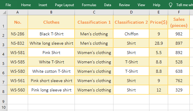
Figure 6

2. Formula description:

Formula =SUM(SUMIFS(F2:F8,C2:C8,"Women's clothing", D2:D8,{"Shirt","T-shirt"})) are combined by Sum and SumIfs, due to the second Criteria {"Shirt","T-shirt"} of SumIfs is an array, and SumIfs can only return the summation value that matches the first Criteria of the array("Shirt") by default. After Sum is added, SumIfs can return the value that meets the two Criteria in the array as an array, ie =SUM({1983;1166}), then add with Sum.

(II) SumIfs function date condition summation

1. If you want the sum of the "Sales" of "Trouser" in January. Select cell C10 and copy the formula =SUMIFS(D2:D9,A2:A9,">=2019/1/1", A2:A9,"<=2019/1/31") to C10, press Enter, return the summation result 1709, the operation process steps, as shown in Figure 7:

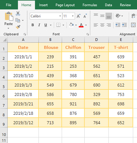
Figure 7

2. The formula =SUMIFS(D2:D9,A2:A9,">=2019/1/1", A2:A9,"<=2019/1/31") Both Criteria_Range are A2:A9, Criteria for ">=2019/1/1" and "<=2019/1/31", it is to find all the dates of January.

3. If the sum of the "Sales" of all garments in January is required, and then SumIfs is not easy to write conditions, the array condition is not good, because the array condition is "OR" rather than "AND", which can use Sum + Month function. The following is a demonstration of using the Sum + Month function to achieve the sum of the "Sales" of "Trouser" in January and the sum of all apparel "Sales" in January, as shown in Figure 8:

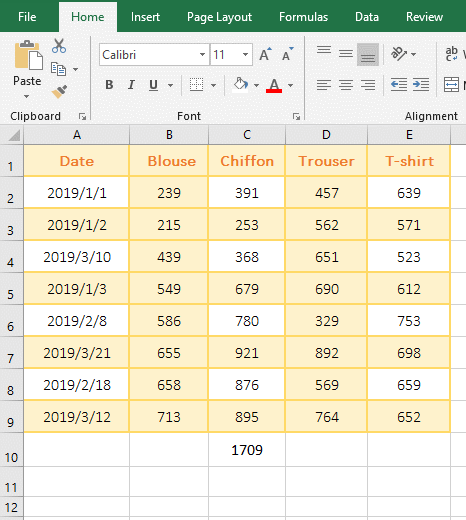
Figure 8

(1) Demonstration: Copy the formula =SUM((D$2:D$9)*(MONTH(A$2:A$9)=1)) to cell C11 cell, press Ctrl + Shift + Enter to return the result 1709; Double-click C11, change D$2 to B$2 and D$9 to E$9, press Ctrl + Shift + Enter to return to the summation result 5857.

(2) Formula description

A. =SUM((D$2:D$9)*(MONTH(A$2:A$9)=1)) is an array formula, so press Ctrl + Shift + Enter.

B. D$2:D$9 returns all the values in D2 to D9 as an array, which returns {456;562;651;690;329;892;569;764}.

C. A$2:A$9 returns all dates in A2 to A9 as an array. MONTH(A$2:A$9)=1 is used to take the month of each date in A2 to A9, and then compare with 1, if equal to 1, Returns True, otherwise returns False; for example, take A2(2019/1/1), MONTH(A1) = 1, and compare with 1, return equal to True, and so on; finally return array {True; True ;False;True;False;False;False;False}.

D. The formula becomes =SUM({456;562;651;690;329;892;569;764}*{True;True;False;True;False;False;False;False}), then the elements that correspond to each other in the two arrays are multiplied. When multiplied, since True is converted to 1, False is converted to 0, the formula becomes =SUM({457;562;0;690;0;0;0;0}), and add finally with Sum.