 Office > Excel > Excel 2019 > Content
Excel lookup function usage(Multiple conditional and approximate/fuzzy lookup)
The LookUp function is divided into a vector form and an array form in excel, where the vector form is used to look up in a column or a row, and the array form is used to look up in an array or multiple columns and multiple rows. The vector form can have three parameters, and the array form can only have two parameters. In general, the VLookUp function or the HLookUp function can be considered when using the array form.
The use of the LookUp function is divided into basic usage methods, multi-condition finding, fuzzy lookup(approximate search), and look up the full name according to the short name. Multi-condition search can find values that satisfy two or more conditions. In case of multiple conditional search, the LookUp function is often used, instead of using the VLookUP function, on the one hand, it is easy to write conditions, on the other hand, the execution efficiency is high.
I, Excel LookUp function syntax
(I) Vector form
1. expression: =LOOKUP(Lookup_Value, LookUp_Vector, [Result_Vector])
2. Description:
A. The LookUp_Vector is an range that can only contain one row or one column, and the values must be sorted in ascending order, otherwise incorrect values may be returned.
B. The Result_Vector is optional and is an range that can only contain one row or one column, and must be the same size as the LookUp_Vector.
C. If the lookup value is not found in the LookUp_Vector, the LookUp function will return the maximum value in the LookUp_Vector that is less than or equal to the lookup value. If the Lookup_Value is less than the minimum value in the LookUp_Vector, the LookUp function will return the #N/A error value.
(II) Array form
1. Expression: =LOOKUP(Lookup_Value, Array)
2. Description:
(1) If the Lookup_Value is not found in the array, the LookUp function will return the maximum value in the array that is less than or equal to the Lookup_Value; if the Lookup_Value is less than the minimum value in the first row or the first column (determined by the array dimension), the LookUp function will return the #N/A error value.
(2) The difference between the array form of LookUp function and VLookUp function and HLookUp function: VLookUp function searches for the Lookup_Value in the first column, HLookUp function searches in the first line, and LookUp function searches according to the array dimension, as follows:
A. If the number of array columns is greater than the number of rows, such as {1,3,5;2,4,6}, the LookUp function will search for the Lookup_Value in the first row.
B. If the number of array rows is greater than or equal to the number of columns, such as {1,3;2,4;8,10}, the LookUp function will search for the Lookup_Value in the first column.
C. Using the VLookUp function and the HLookUp function, you can search down or traverse the search by index, while the LookUp function always selects the last value in the row or column; therefore, if you use the array form of the LookUp function, it is recommended to use the VLookUp function or the HLookUp function.
(3) The values in the array must also be sorted in ascending order, otherwise incorrect values may be returned.
II, The use of Excel LookUp function one: vector form
(I) Values must be sorted in ascending order and the LookUp_Value(fuzzy lookup) cannot be found in the LookUp_Vector
1. If you want to find sales by price. Select A11 cell, enter the LookUp_Value 8, double-click B11, copy formula =LOOKUP(A11,D2:D8,E2:E8), and paste it in B11, press Enter, return to 892; select D2:D8, select "Data" tab, click the "ascending(A→Z)" icon, select "Extended the Selected" in the "Sort Warning" window that opens, click "Sort", then each row is sorted in ascending order of "price", and the value in B11 also becomes 528; operation process steps, as shown in Figure 1:
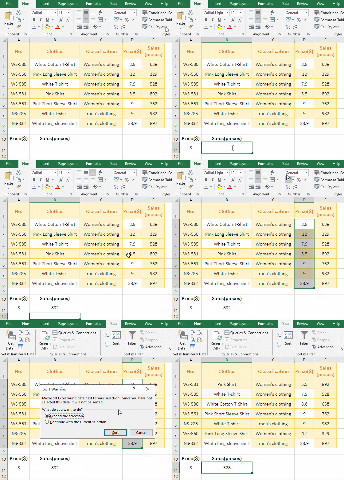
Figure 1
2. Description:
In formula =LOOKUP(A11,D2:D8,E2:E8), A11 is the LookUp_Value, D2:D8 is the LookUp_Vector, E2:E8 is the Result_Vector; the first return 892 is the incorrect return value because the LookUp function requires values in Lookup_Vector to be sorted in ascending order. After sorting the prices in ascending order, the correct LookUp_Value 528 is returned, because if the LookUp_Value is not found, the LookUp function will return the maximum value(ie, the approximation) that is less than or equal to the LookUp_Value in the LookUp_Vector, 79.9 is exactly the value.
(II) The LookUp_Value is less than the minimum value in the LookUp_Vector, and the #N/A error value is returned.
The lowest price for clothing is 5.5, if you want to find the clothing sales with a price of 5. Select A11 cell, enter 5, double-click B11, copy formula =LOOKUP(A11,D2:D8,E2:E8), and paste it in B11, press Enter, return #N/A error value; operation process step, as shown in Figure 2 Show:
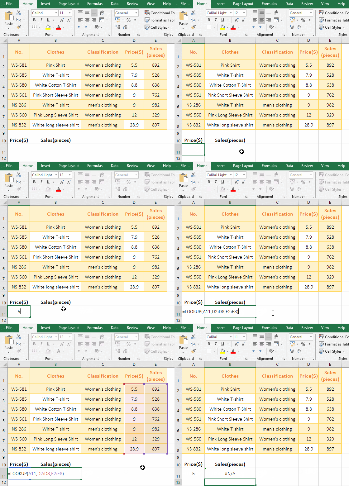
Figure 2
(III) Cannot find the value to return the last row
1. If you want to find the name "Red T-shirt" that doesn't have in the "Clothes" and return to the "Sales". Double-click the A11 cell, enter the "Red T-Shirt", double-click B11, copy the formula =LOOKUP(A11,B2:B8,E2:E8), and paste it in B11, press Enter, return to 329; the operation steps, as shown in Figure 3 Show:
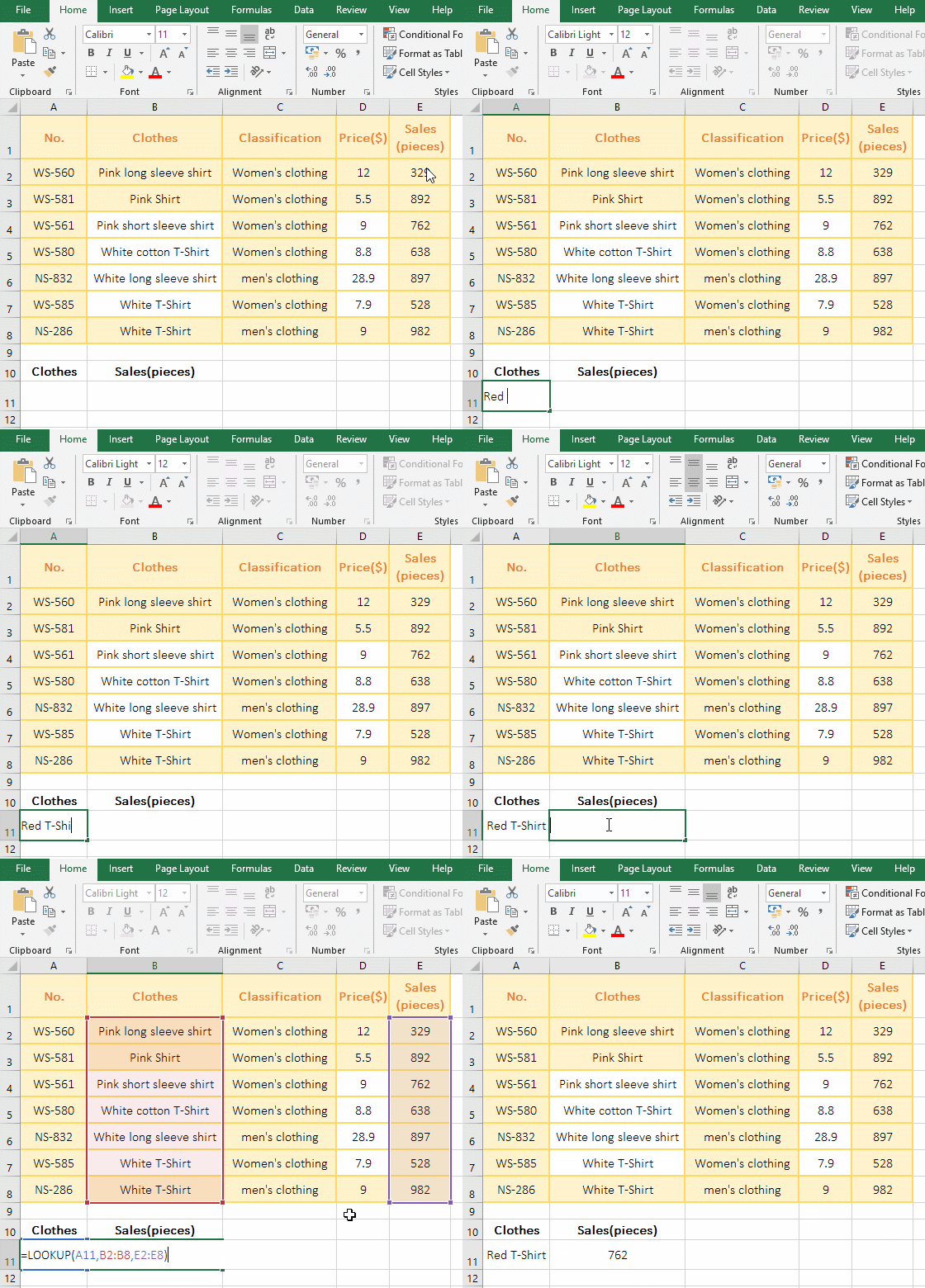
Figure 3
2. There is no "Red T-Shirt" in the "Clothes", so LookUp returns to the maximum value that is less than or equal to the LookUp_Value in the LookUp_Vector, which returns the sales volume 762 corresponding to the "Pink short sleeve shirt".
Hint: The values in Lookup_Vector must be sorted in ascending order.
III, The use of Excel LookUp function two: array form
(I) Search range is an array (The number of columns is greater than the number of rows)
1. Select cell A1, copy the formula =LOOKUP(3,{2,3,5;8,10,15}), paste it in A1, press Enter, return to 10, and the operation steps are as shown in Figure 4:
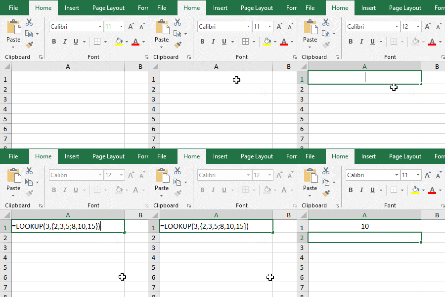
Figure 4
2. The Lookup_Value of formula =LOOKUP(3,{2,3,5;8,10,15}) is 3, the search range is an array; because the number of columns of the array is greater than the number of rows, so look in the first row, after find Returns 10 of the corresponding column.
(II) Search range are cells (the number of rows is greater than or equal to the number of columns)
1. Double-click cell A11 and enter the "Black T-Shirt"; double-click B11, copy the formula =LOOKUP(A11,B2:E8), and paste it in B11, press Enter, return to 982; double-click B11, change E8 to E4, press Enter and return to the "Pink T-shirt"; the process steps, as shown in Figure 5:
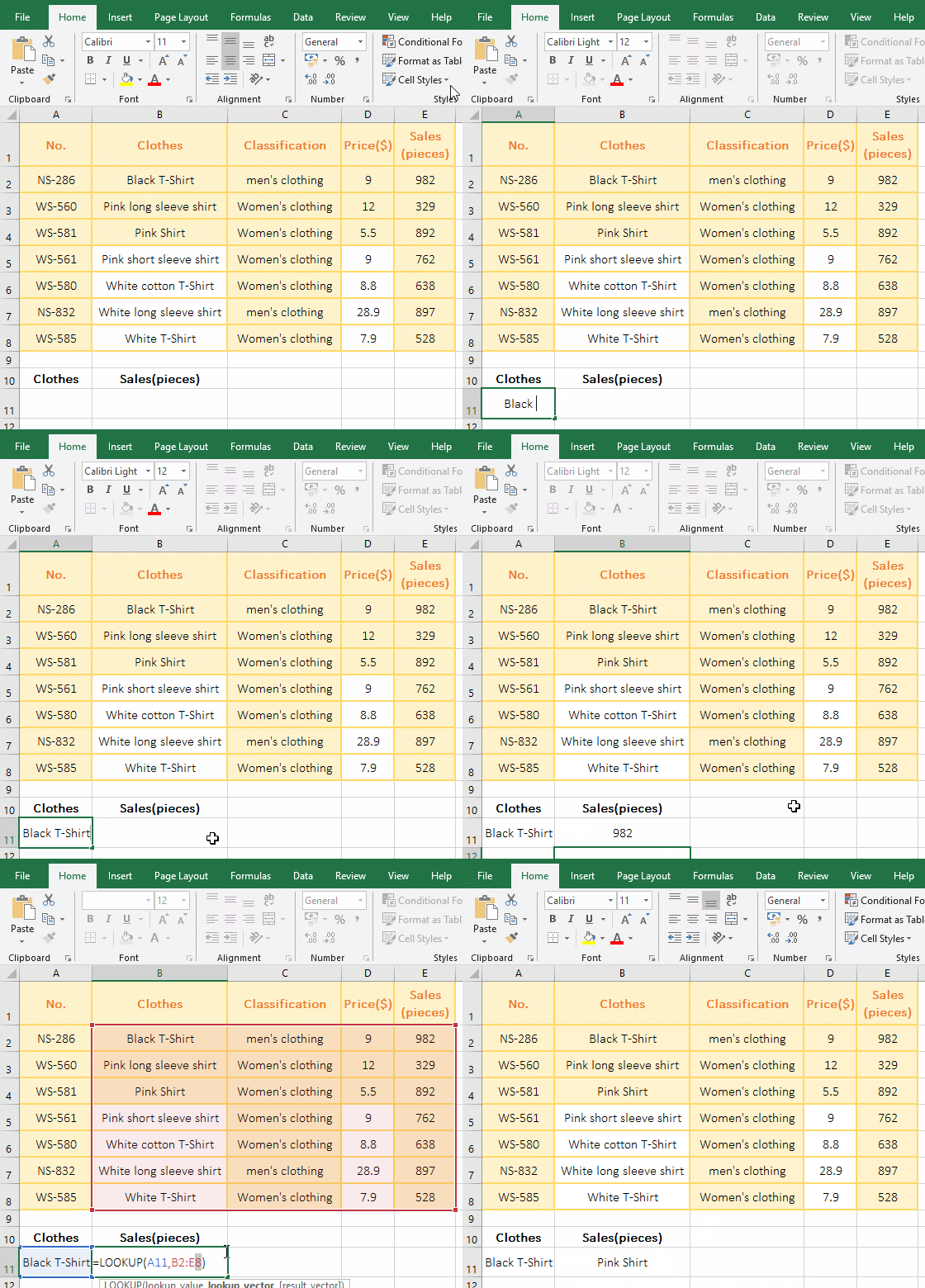
Figure 5
2. Formula =LOOKUP(A11,B2:E8) search range is B2:E8, which belongs to the case which the number of rows is greater than the number of columns, find in the first column, find in B8, and then return to the value 982 that corresponds to B8 in the last column (ie column E); the search range of formula =LOOKUP (A11,B2:E4) is B2:E4, which belongs to the case which the number of rows is equal to the number of columns (ie, 4 rows and 4 columns), and is also found in the first column, since it is not found, Returns the value of the last row.
IV, The use of Excel LookUp function three: extend the application
(I) Multiple conditional search
1. If you want to find the name of the clothing classified is "Women's clothing" and its price is 8.8. Double-click cell A11, type "women's clothing", select B11, enter 8.8, double-click C11, and put the formula =LOOKUP(1,0/((C2:C8=A11)*(D2:D8=B11)),B2:B8) Copy to C11, press Enter, return to the "White cotton T-Shirt", the operation steps, as shown in Figure 6:
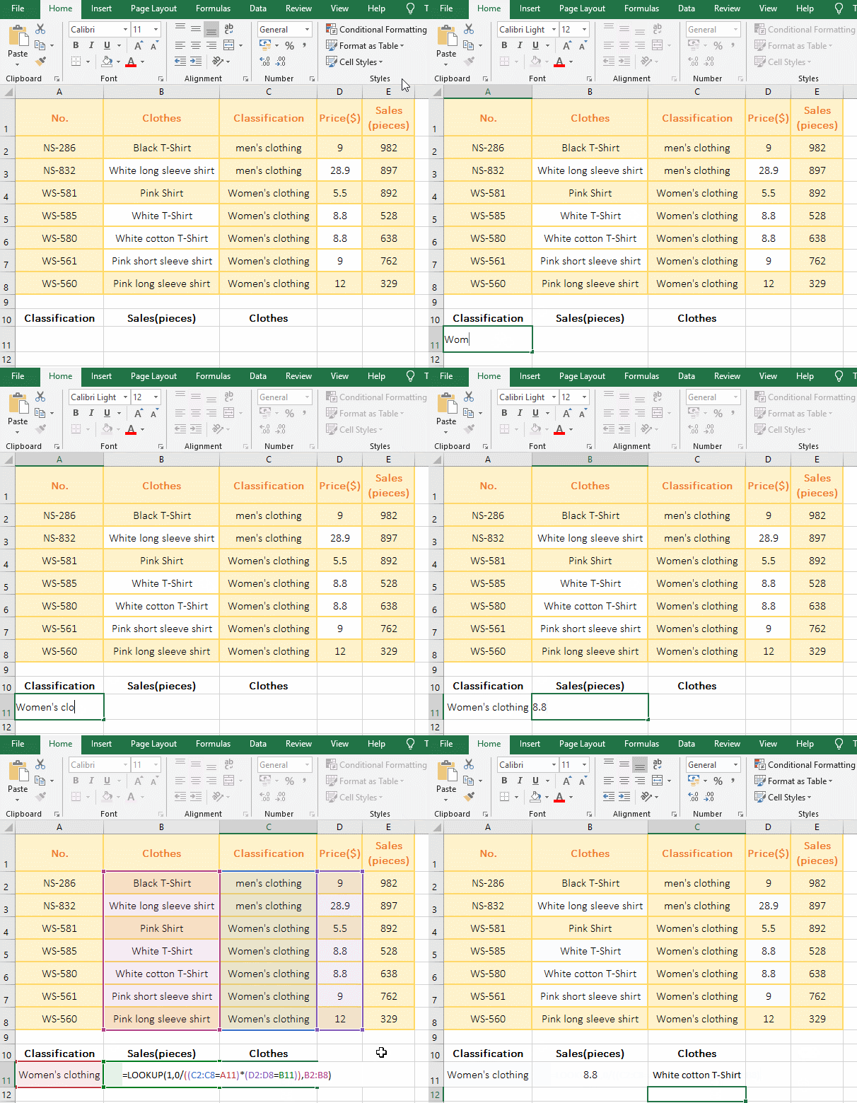
Figure 6
2. Formula =LOOKUP(1,0/((C2:C8=A11)*(D2:D8=B11)),B2:B8) Explanation:
A. C2:C8=A11 is the condition, C2:C8 returns the data of C2 to C8 in the form of an array, that is, {"men's clothing"; "Women's clothing";"Women's clothing"; "Women's clothing"; "Women's clothing"; "Women's clothing"; men's clothing; "Women's clothing"}; when executed, first take the first element "men's clothing" from the array, it is not equal to A11 (Women's clothing), return false, the second time to take out the second element "Women's clothing" from the array, it equals to A11, return True; the other and so on, and finally return {FALSE; FALSE; TRUE; TRUE; TRUE; TRUE; TRUE}.
B. The same reason D2:D8=B11 return array {FALSE; FALSE; FALSE; TRUE; TRUE; FALSE; FALSE}, then (C2:C8=A11)*(D2:D8=B11) becomes {FALSE; FALSE; TRUE; TRUE; TRUE; TRUE; TRUE}*{FALSE; FALSE; FALSE; TRUE; TRUE; FALSE; FALSE}, multiplies the corresponding elements of the two arrays, and True is multiplied by 1 , FALSE is converted to 0, and finally returns {0; 0; 0; 1; 1; 0; 0}.
C. Then 0/((C2:C8=A11)*(D2:D8=B11)) becomes 0/{0; 0; 0; 1; 1; 0; 0}, followed by 0 divided by each element of the array, the result is {#DIV/0; #DIV/0; #DIV/0; 0; 0; #DIV/0; #DIV/0}.
D. The formula becomes =LOOKUP(1,{#DIV/0; #DIV/0; #DIV/0; 0; 0; #DIV/0; #DIV/0},B2:B8 ), then look for 1 in the array, because there is no 1 in the array, so return a maximum value less than or equal to 1, that is, return 0, and because the LookUp function is to select the last value that meets the condition, so find the second 0 (ie D6), and finally return the "Clothes" "White cotton T-Shirt" that correspond to D6 in B6 in column B.
Hint: The values in C and D column must be sorted in ascending order. If you don't know the sort, Please refer to the article "How to sort in excel(11 examples), include sort by column,color,date,row and use shortcut keys".
(II) Excel fuzzy lookup(Approximate search)
1. If you want to return the "Grade Scale" of each student based on the average score. Double-click cell F2, copy the formula =LOOKUP(E2,{0,60,70,80,90;"F","D","C","B","A"}), and paste it in F2, press Enter, return to the first student's Grade Scale "B"; select F2, move the mouse to the cell fill handle on the lower right corner of F2, double-click the left button to return the Grade Scale of the remaining students; the operation steps, as shown in Figure 7:
Figure 7
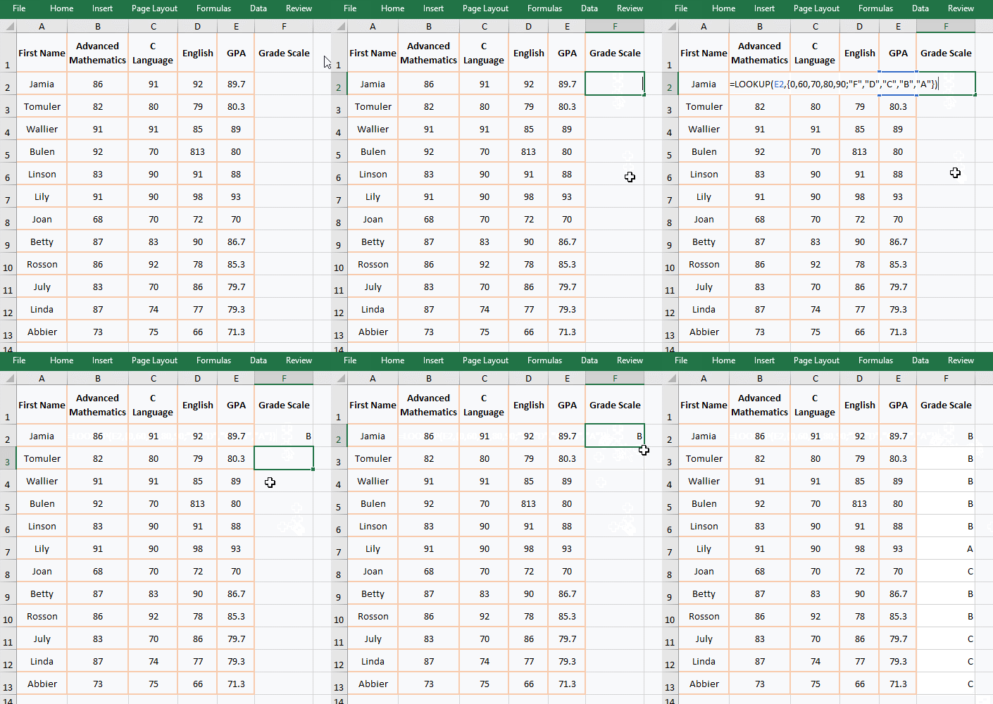
2. Formula description:
The Look_Vector of formula =LOOKUP(E2,{0,60,70,80,90;"F","D","C","B","A"}) is a array of 5 columns and 2 rows. When looking up F2 (89.7), since it is not found in the first line, select the maximum value less than or equal to 89.7, that is, select 80, and then return the value of the fourth column corresponding to B, and so on.
(III) Find the full name according to the abbreviation
1. If you want to find the full name of the supplier based on the supplier's short name. The current sheet is "Supplier", click "Ingoods" to switch to the sheet, double-click cell D2, copy the formula =IFERROR(LOOKUP(1,0/FIND(B2,Supplier!A$2:A$7),Supplier!A$2:A$7),""), paste it in D2, press Enter, return to the full name of B2; select D2, move the mouse to the cell fill handle on the lower right corner of D2, double click the left button to return the remaining full name of the garment supplier; the operational process steps, as shown in Figure 8:
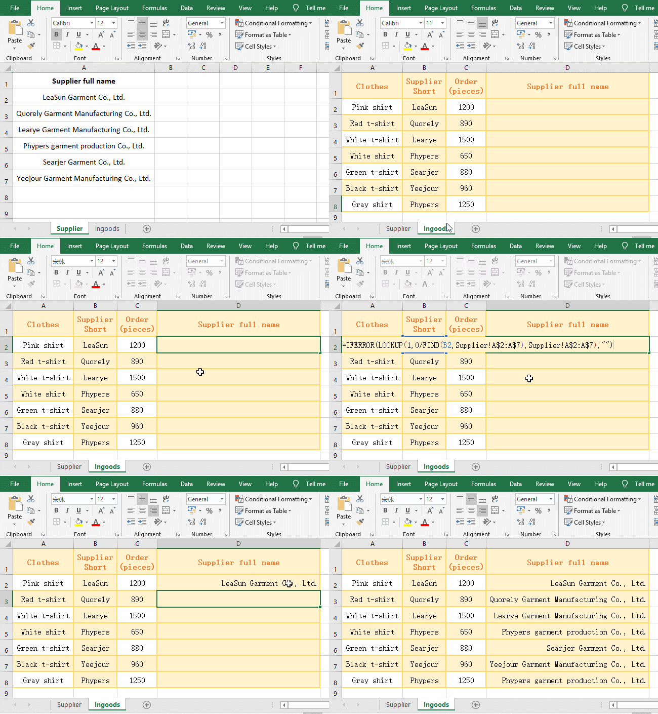
Figure 8
2. Formula =IFERROR(LOOKUP(1,0/FIND(B2,Supplier!A$2:A$7),Supplier!A$2:A$7),"")
A. "Supplier" that is in "Supplier!A$2:A$7" is the name of the sheet, A$2 means absolute reference to the column and relative to the row, when dragging down, the column and row number are unchanged, that is, A2 will not Change to A3, A4, ...; A$7 and A$2 are a meaning; A$2:A$7 returns the data in A2 to A7 as an array, ie {"LeaSun Garment Co., Ltd."; "Quorely Garment Manufacturing Co., Ltd."; "Learye Garment Manufacturing Co., Ltd.";"Phypers garment production Co., Ltd."; "Searjer Garment Co., Ltd."; "Yeejour Garment Manufacturing Co., Ltd."}.
B. Then FIND(B2,Supplier!A$2:A$7) becomes FIND(B2,{"LeaSun Garment Co., Ltd."; "Quorely Garment Manufacturing Co., Ltd."; "Learye Garment Manufacturing Co., Ltd.";"Phypers garment production Co., Ltd."; "Searjer Garment Co., Ltd."; "Yeejour Garment Manufacturing Co., Ltd."}), B2 is "LeaSun", use Find function to find B2 in the array, find returned 1, failed to find return the value error #VALUE!, and finally returned {1;#VALUE!;#VALUE!;#VALUE!;#VALUE!;#VALUE!}.
C. Then 0/FIND(B2,Supplier!A$2:A$7) becomes 0/{1;#VALUE!;#VALUE!;#VALUE!;#VALUE!;#VALUE!}, then each element in the array divided by 0 and finally return {0;#VALUE!;#VALUE!;#VALUE!;#VALUE!;#VALUE!}.
D. The formula becomes =IFERROR(LOOKUP(1,{0;#VALUE!;#VALUE!;#VALUE!;#VALUE!;#VALUE!,Supplier!A$2:A$7),""). Then, use LookUp function to find 1 in the array, and also if don't find, it will return the maximum value less than or equal to 1, that is, return 0(that is, A2 in the "supplier").
E. The IfError function is used for error handling, and if LookUp returns an error, it returns a null value, otherwise it returns the return value of LookUp.
-
Related Reading
- How to set Header and footer in word(13 examples), i
- How to start page numbers on page 3 and each section
- VLookUp in excel introduces step by step(10 examples
- Excel If function examples, include if statement nes
- How to find duplicate values in excel using vlookup(
- Excel SumIf function with ?/*, Average and array mul
- Vlookup with if statement(use if/if{0,1} combination
- The use instances of Excel Round function, include R
- How to sort in excel(11 examples), include sort by c
- How to wrap text in excel and displays paragraph in
- How to sum in excel(9 formulas), include sum use sho
- How to create drop down list in excel and update/del