How to use hlookup in excel(7 hlookup example, combine Match function)

In Excel, The VLookUp and LookUp functions are used for straight lookup, while the HLookUp function is used for horizontal lookup, which are usually found in the first row of the table, but if the selected range does not include the first row of the table, it is not found in the first row of the table.

When searching for values, letters, and logical values and matching options are set to fuzzy matches, you need to sort the first line of the search range, otherwise the HLookUp function may return incorrect results; when no value is found, the HLookUp function returns the wrong value. The HLookUp function can be used in combination with the Match function to dynamically return values for different rows.

I, Excel HLookUp function syntax

1, expression: HLOOKUP(LookUp_Value, Table_Array, Row_Index_Num, [Range_LookUp])

2. Description:

A. LookUp_Value needs to find in the first row of the selected range. If the selected range does not include the first row of the table, it is not found in the first row of the table; for example, if the selected range is B2:C9, it should be Look for LookUp_Value in B2:C2, which means that B2:C2 is the first row, so don't think of the first row of the table as a lookup line.

B. If Range_Lookup is set to True, the value, letter, and logical value of the first row in Table_Array must be in ascending order from left to right, otherwise HLookUp may return an incorrect value; if Range_LookUp is set to False, Table_Array does not need to be sorted; The text in Table_Array is not case sensitive.

C. When Row_Index_Num is 1, the value of the first row in Table_Array is returned; when Row_Index_Num is 2, the value of the second row in Table_Array is returned; the others and so on. If Row_Index_Num is less than 1, HLookUp returns the wrong value #VALUE!; if Row_Index_Num is greater than the number of rows in Table_Array, HLookUp returns the reference error value #REF!.

D. Range_LookUp is optional, it has two options, one is True (approximate match), the other is False (exact match); if Range_LookUp is omitted or True, if LookUp_Value is not found, it returns less than the maximum value of LookUp_Value. If Range_LookUp is False, if LookUp_Value is not found, the error value #N/A is returned.

E. If Range_LookUp is set to False and LookUp_Value is text, the wildcard question mark (?) and asterisk (*) can be used in LookUp_Value; the question mark matches any character, the asterisk matches any one or a string of characters; if you want to find the question mark Or asterisk, you need to add the escape character ~, for example to find the question mark, you should write ~?, the asterisk should be written like this ~ *.

I, The use of Excel HLookUp function

(I) Omitting the parameter Range_LookUp

1. If you want to find "First Name" in the first row. Double-click the A10 cell, copy the formula =HLOOKUP("First Name",A1:C9,5), paste it in A10, press Enter, return to the "Finance"; double-click A10, add a comma(,) after 5, press Enter. return to "Fulinter"; double-click A10, enter "true" after the comma, press Enter, return to "Finance"; double-click A10 again, change true to false, press Enter, return to "Fulinter"; operation steps, as shown in Figure 1. Shown as follows:

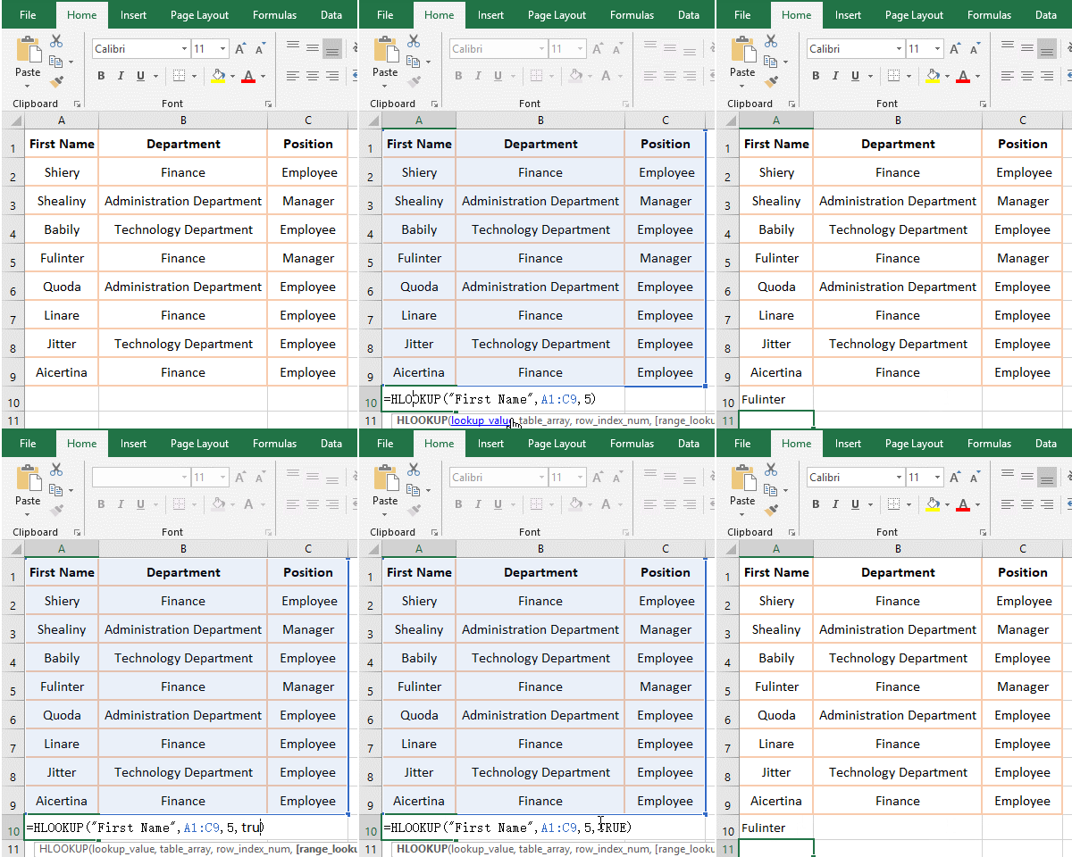
Figure 1

2. Formula description:

A. Formula =HLOOKUP("First Name",A1:C9,5), "First Name" is the LookUp_Value, A1:C9 is the Table_Array, 5 is the Row_Index_Num, the formula omits the parameter Range_LookUp; the meaning of the formula is that looks for "First Name" in the first row(the first row of the designated range A1:C9) and returns the value in row 5.

B. Formula =HLOOKUP("First Name",A1:C9,5) and =HLOOKUP("First Name",A1:C9,5,true) are returned to the "Finance", indicating that the third parameter 5 is not followed by a comma, the parameter Range_LookUp selects True by default; the formula =HLOOKUP("First Name",A1:C9,5) and =HLOOKUP("First Name",A1:C9,5,false) both return "Fulinter", indicating the third parameter 5 followed by a comma, Range_LookUp selects False by default.

(II) The parameter Row_Index_Num is less than 1 and larger than the number of rows in the Table_Array

1. Double-click cell A10, copy the formula =HLOOKUP("First Name", A1:C9,0,1), paste it in A10, press Enter, return the value error #VALUE!; double-click A10, change 0 to 9, press Enter, return "Finance"; double-click A10 again, change 9 to 10, press Enter, return reference error #REF!; operation process steps, as shown in Figure 2:

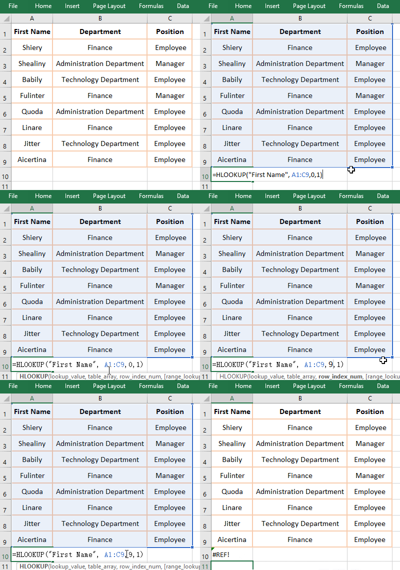
Figure 2

2. Formula description:

In the formula =HLOOKUP("First Name", A1:C9,0,1), the return Row_Index_Num is 0, it returns value error #VALUE!, indicating that Row_Index_Num is less than 1, it returns value error; when 0 is changed to 9, it returns the value in row 9; when 9 is changed to 10, Row_Index_Num has exceeded the maximum number of rows in the selected range, thus it returns a reference error.

(III) Cannot find LookUp_Value, return the maximum smaller than LookUp_Value(the first row in the Table_Array needs to be sorted)

1. If you want to find sales volume 589. Double-click cell B10, copy the formula =HLOOKUP(589,B2:E9,4,TRUE) to B10, press Enter to return to 612; double-click E2, change 567 to 639, and the return value in B8 becomes 690. The process steps are shown in Figure 3:

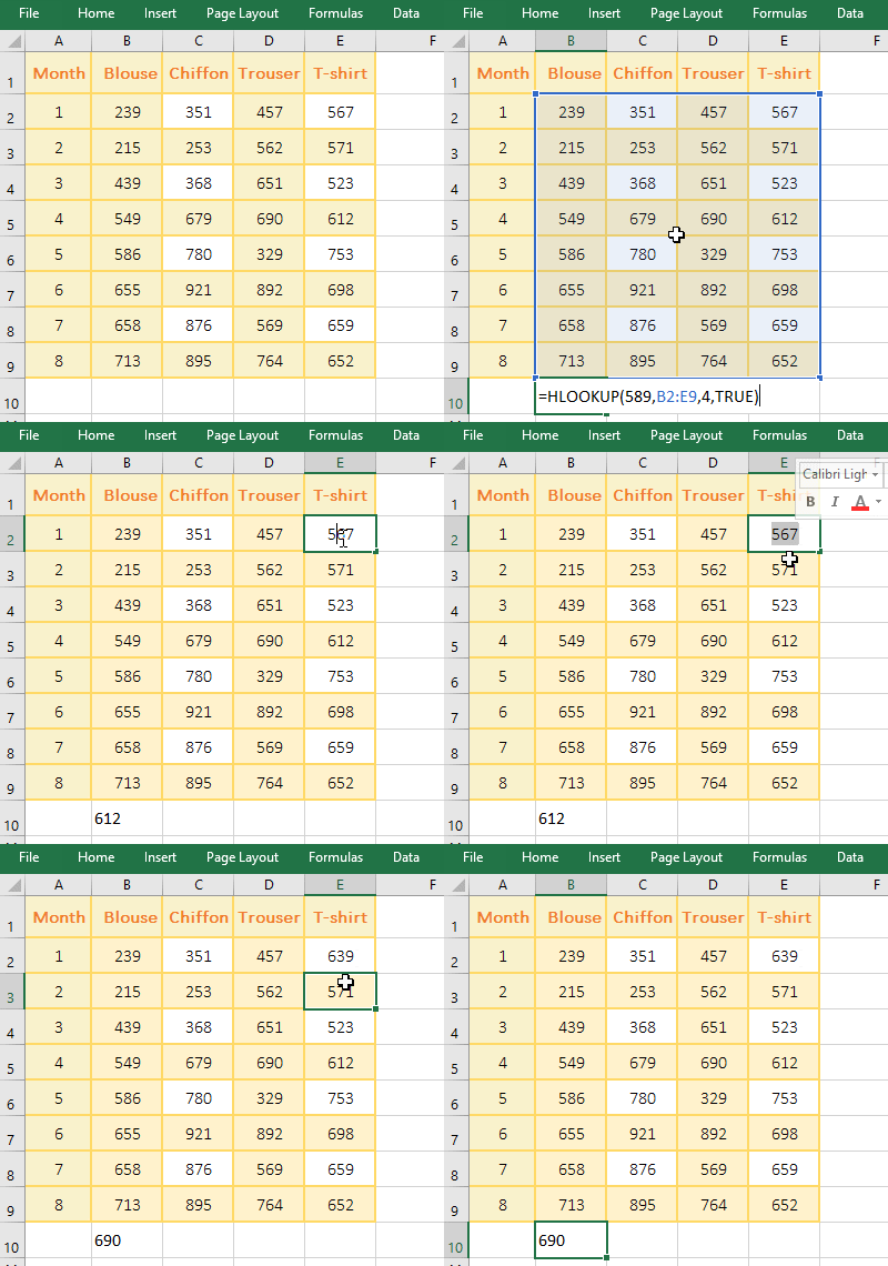
Figure 3

2. Formula =HLOOKUP(589,B2:E9,4,TRUE) Description:

B2:E9 is the Table_Array, the first row here refers to B2:E2 (that is, the first row of the non-form), that is, find 589 in the second row of the table; since 589 is not found, the value 551 that is the maximum less than or equal to 589 was returned, then return the value 612 in the fourth row of the column; since the Range_LookUp is set to True here, the search for rows B2:E2 needs to be sorted from left to right in ascending order, otherwise incorrect values may be returned. After changing 567 to 639, the return value becomes 690, because 589 is less than 639, returning a value less than 589 is only 457, and then returns the value in row 4 of the same column, so it returns 690.

(IV) Cannot find LookUp_Value, return the wrong value #N/A(The first row of the Table_Array does not need to be sorted)

1. Also look for sales volume 589. Double-click cell B10, copy the formula =HLOOKUP(589,B2:E7,4,FALSE) to B10, press Enter, return the numeric error value #N/A; double-click C10, change 591 to 391, the value in B10 Still #N/A; the operation process steps, as shown in Figure 4:

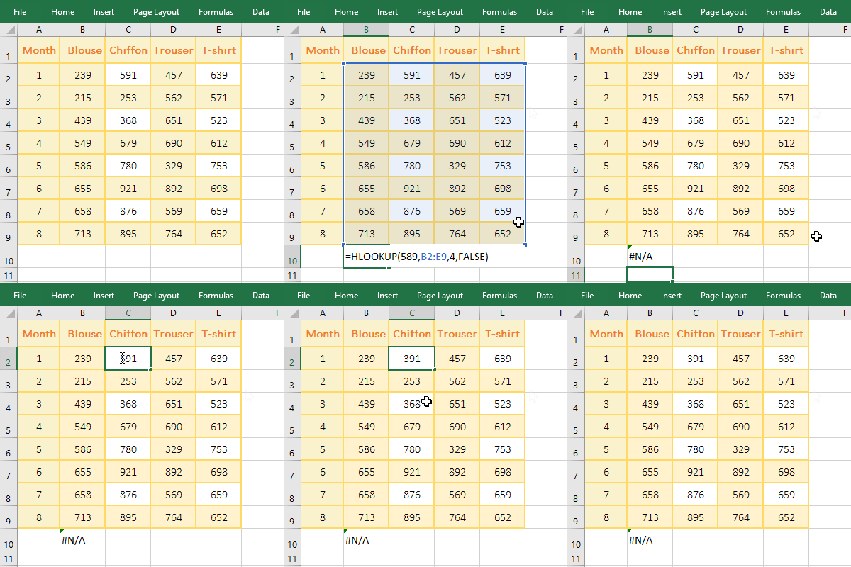
Figure 4

2. Formula =HLOOKUP(589,B2:E9,4,FALSE) Description:

On the first execution, the search row B2:E2 is not sorted in ascending order from left to right, the formula returns the error value #N/A; when 591 is changed to 391, the search row B2:E2 has been sorted in ascending order, but the value in B10 is still the error value #N/A, indicating that whether the search row is sorted or not sorted in ascending order, when the Range_LookUp parameter is set to False, if the LookUp_Value is not found, the HLookUp function returns the error value #N/A, that is, when it is the exact match, the search row without sorting.

(V) Examples of Lookup_Value with wildcard questions (?) and asterisks (*)

1. The Lookup_Value has a wildcard problem (?)

A. If you want to find sales that start with any 5 characters and end with "Shirt". Double-click cell B4, copy the formula =HLOOKUP("?????Shirt", B1:F3,3,FALSE) to B4, press Enter, return to 892, and proceed as shown in Figure 5:

Figure 5

B. Formula =HLOOKUP("?????Shirt", B1:F3,3,FALSE) "????? Shirt" is the Lookup_Value, a question mark indicates a character, meaning to start with any 5 characters and end with "Shirt". There are wildcards in the lookup value, and the Range_LookUp parameter needs to be set to False.

2. The Lookup_Value has a wildcard asterisk (*)

A. If you want to find sales that start with any character and end with a "T-Shirt." Double-click cell B4, copy the formula =HLOOKUP("*T-Shirt", B1:F3,3,FALSE) to B4, press Enter, return to 982; double-click B4 again, change "*T-Shirt" to "*White*", press Enter, return to 897; operation steps, as shown in Figure 6:

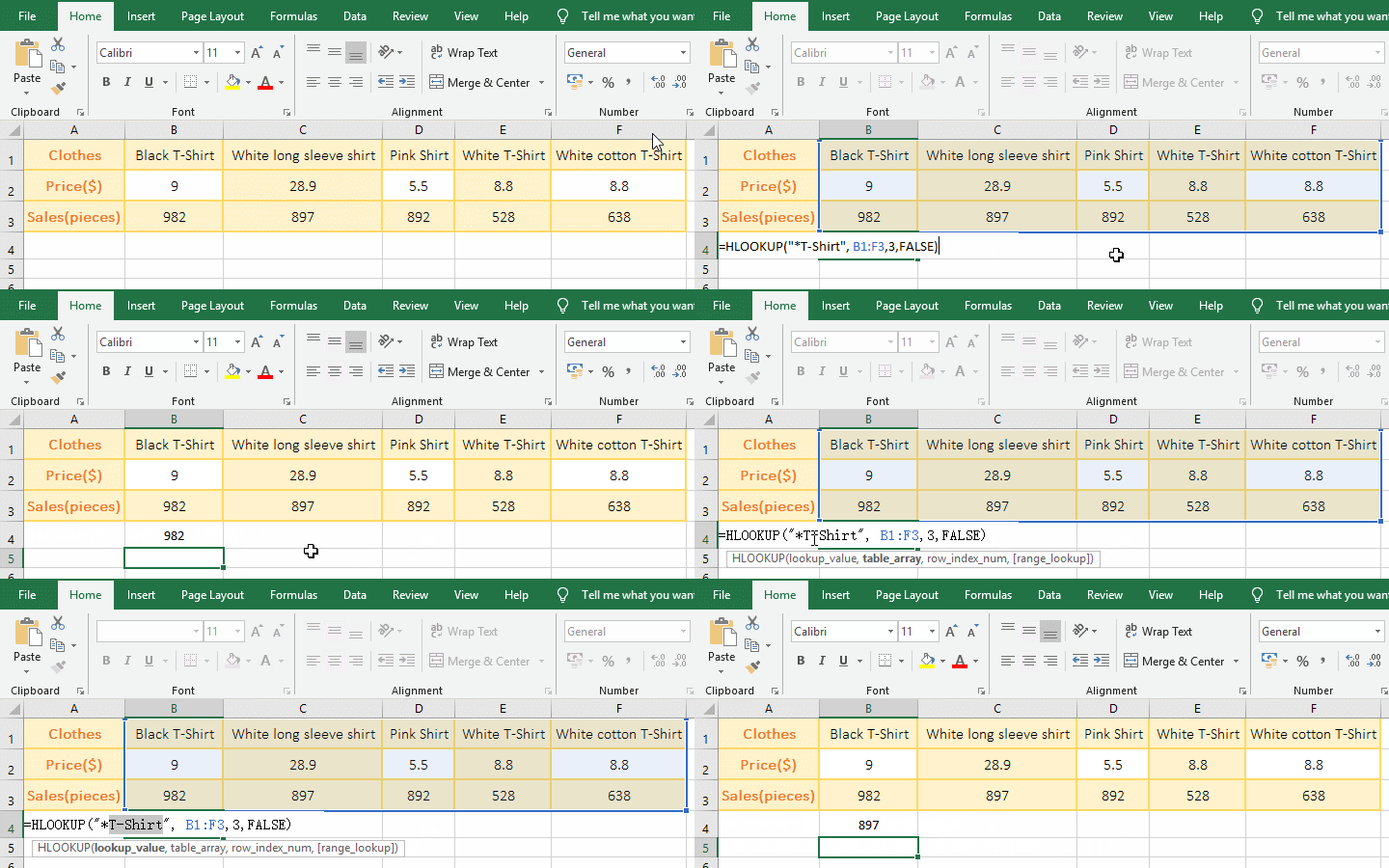
Figure 6

B. "*T-Shirt" is a Lookup_Value in formula =HLOOKUP("*T-Shirt", B1:F3,3,FALSE), meaning that it starts with any one or more characters and ends with "T-Shirt", the values n D1 and E1 are all eligible, but the HLookUp function selects the first value that meets the condition, so it returns 982; after changing "*T-Shirt" to "*White*", the values in C1 and E1 and F1 are eligible, also Select the first value that meets the criteria, so return 897.

III, Excel combine HLookUp + Match and non-first row instance

1. If you want to find the "May Sales(pieces)" of "White T-Shirt". Double-click cell F8 and copy the formula =HLOOKUP($F$7,A1:D5,MATCH($E$8,A1:A5,0),0) to F8, press Enter, return to 780; right-click the first row number 1, in the pop-up menu, select "Insert", then insert a row in the first row, the row where the formula is located will also move down automatically, F8 will change to F9, and each reference cell in the formula will also be automatically incremented by 1. The value in F9 is still 780; operation process steps, as shown in Figure 7:

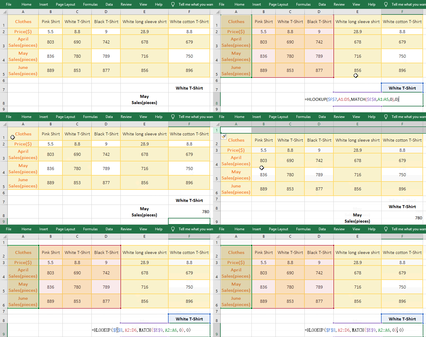
Figure 7

2. Formula =HLOOKUP($F$7,A1:D5,MATCH($E$8,A1:A5,0),0) Description:

A. $F$7 is an absolute reference to the cell F7, that is, whether it is dragging down or dragging to the right, F7 will not become F8, F9, ... or G8, H8, ..., but when inserting rows, $F$7 will automatically change to $F$8; $E$8 and $F$7 are a meaning.

B. MATCH($E$8,A1:A5,0) is to find E8 (ie "May Sales(piece)") in A1:A5, 0 means exact match, and finally returns 4.

C. The formula becomes =HLOOKUP($F$7,A1:D5,4,0), then look for the "White T-shirt" in the first row, found in C1, return the value in the fourth row of the column , exactly 780; the last parameter of the HLOOKUP formula 0 means exact match.

D. After inserting a row in the first row, the formula becomes =HLOOKUP($F$8,A2:D6,MATCH($E$9,A2:A6,0),0), and the Table_Array becomes A2:D6, the first row also becomes A2:F2, which is the second row of the table.

Hint: If you want to drag down, the formula A1:D5 will become an absolute reference, ie $A$1:$A$5, the formula becomes =HLOOKUP($F$7,$A$1:$D$5,MATCH($E$8, A1:A5, 0), 0).