How to use excel aggregate function(ignore error values, null values for sum, average)

The Aggregate function is one of the new functions in Excel 2010. It is used to ignore error values, null values, hidden rows and columns, subtotal function subtotal summation, averaging, counting cells, finding maximum and minimum values. The Aggregate function is divided into reference form and array form. It support 19 functions; there is at least one reference, and there can be at most 253; the array form only supports 6 functions, and k argument is required.

The main function of the Aggregate function is to ignore the error value, null value, hidden row and column. If the corresponding function summation, averaging, etc. can not achieve this purpose, you can use the Aggregate function, which is not only easy to write formulas and make the problem simple.

I, Excel Aggregate function syntax

(1) Reference form

Expression: AGGREGATE(Function_Num, Options, Ref1, [Ref2], ...)

(2) Array form

Expression: AGGREGATE(Function_Num, Options, Array, [k])

(3) Description:

1. Function_Num is the function number, its ranges are 1-19, each number represents a function, as follows:

Function_num                 Function
 
           1                                AVERAGE
 
          2                                   COUNT
 
          3                                  COUNTA
 
         4                                      MAX
 
          5                                     MIN
 
          6                                 PRODUCT
 
         7                                   STDEV.S
 
         8                                  STDEV.P
 
        9                                     SUM
 
       10                                   VAR.S
 
       11                                   VAR.P
 
       12                                  MEDIAN
 
       13                                MODE.SNGL
 
       14                                     LARGE
 
       15                                    SMALL
 
       16                               PERCENTILE.INC
 
       17                                QUARTILE.INC
 
       18                               PERCENTILE.EXC
 
       19                                QUARTILE.EXC

2. Options is the ignore option, there are 0 - 7 eight values, as follows:

0 or omitted: ignore nested Subtotal and Aggregate functions;

1: Ignore hidden rows, nested Subtotal and Aggregate functions;

2: Ignore error values, nested Subtotal and Aggregate functions;

3: Ignore hidden rows, error values, nested Subtotal and Aggregate functions;

4: Ignore nothing;

5: Ignore hidden rows;

6: Ignore the error values;

7: Ignore hidden rows and error values.

3. Ref has at least one, at most 253; if 3D cell are referenced, the value error #VALUE! will be returned.

4. If you use the array form of the Aggregate function, some functions cannot omit the argument K. These functions are Large(Array, k), Small(Array, k), Percentile.inc(array, k), Quartile.inc(Array, Quart)), Percentile.exc(Array, k), Quartile.exc(Array, Quart), if the argument K is omitted, the value error #VALUE! will be returned.

5. When using the Aggregate function for subtotaling, hidden columns are still counted in the subtotal, and hidden rows are not counted.

II, The use of Excel Aggregate function

(I) Ignore nested Subtotal function

1. Double-click cell E9, copy the formula =SUBTOTAL(9,E2:E8) to E9, press Enter, return to the summation result 5028; double-click the E9 cell again, and copy the formula =AGGREGATE(9,0,E2:E9) to E10, press Enter, return to the summation result 5028; the operation steps, as shown in Figure 1:

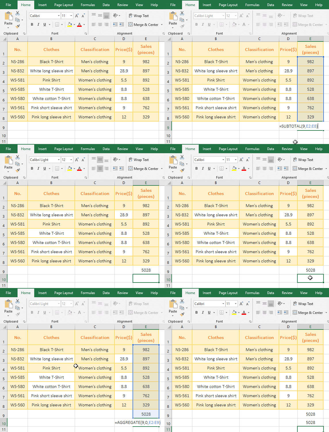
Figure 1

2. The formula =SUBTOTAL(9,E2:E8) is the sum of E2: E8, the formula =AGGREGATE(9,0,E2:E9) to E10 is the sum of E2:E9, the two formulas return the same result, indicating when the Aggregate function Setting the argument Options to 0 ignores the summation result of the Subtotal function.

(II) Ignoring null values

1. Double-click the cell E9 cell, copy the formula =AGGREGATE(9,4,E2:E8) to E9, press Enter to return to the summation result 5028; select E6, press the Delete key to delete the value, and the value in E9 will change 4390; operation process steps, as shown in Figure 2:

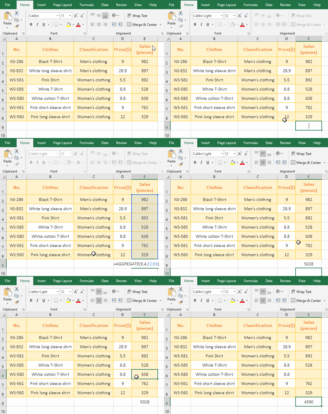
Figure 2

2. When the value in E6 is deleted, the summation result becomes smaller, indicating that when the argument Options is set to 4, the Aggregate function ignores the null value.

(III) Ignore hidden rows but contain hidden column

1. Double-click the cell E9, copy the formula =AGGREGATE(2,5,D2:E8) to E9, press Enter, return to the statistical result 14; right click the second row number 2, select "Hide" in the pop-up menu, the second row is hidden, the statistical result in E9 becomes 12; right click D column number D, select "hidden" in the pop-up menu, hide column D, the value in E9 is still 12; operation process Steps, as shown in Figure 3:

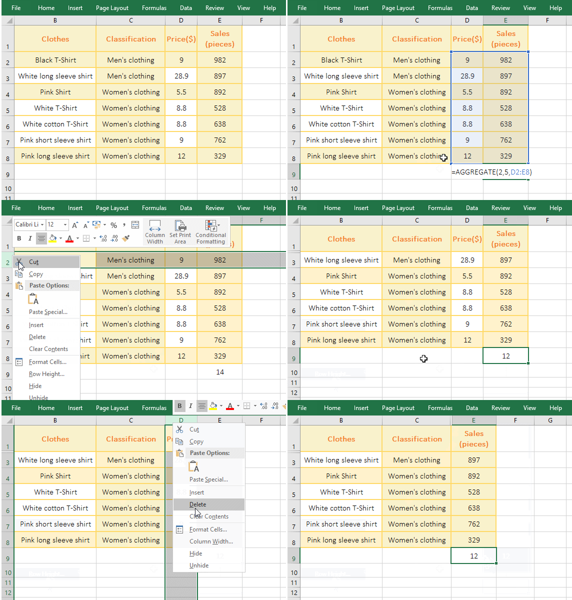
Figure 3

2. 2 represents the function Count that count the number of cells in the formula =AGGREGATE(2,5,D2:E8), 5 means to ignore the null value; when the second row is hidden, the statistical result is reduced by two, indicating that the argument Options is set to 5, the Aggrerate function ignores hidden row; when the column is hidden, the statistics are unchanged, indicating that the Aggrerate function contains hidden columns.

(IV) Ignore the error value

1. If you want to sum up the turnover. Double-click the cell F9, copy the formula =AGGREGATE(9,6,F2:F8) to F9, press Enter, return to the summation result 51896.1; double-click G12, enter the formula =SUM(f2:f8), press Enter, return Value error #VALUE!, double-click G12 again, change f2 to f3, press Enter, also return the summation result 2682664.1; the operation process steps, as shown in Figure 4:

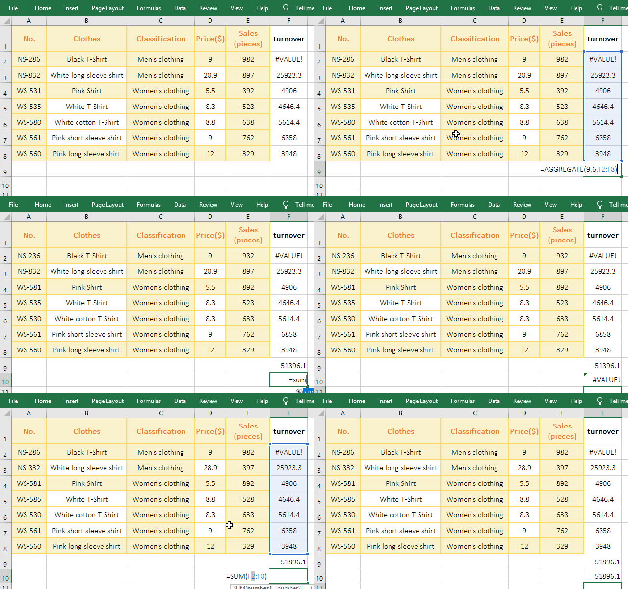
Figure 4

2. 6 means ignore the error value in the formula =AGGREGATE(9,6,F2:F8), the Sum_Range is F2:F8, the value in G2 is an error value, but is ignored; if you use the Sum function, return the value error #VALUE!, only the error value is not included to return the correct result.

Hint: Other functions (such as the averaging function Average, the statistical function Count, CountA, the multiplication and division function Product, the maximum function Max, the minimum function Min, etc.) also support the ignoring of the error value calculation.

(V) An error is returned after the function that requires the argument K that is omitted.

1. If you want to return to the third sales minimum. Double-click the cell E9, copy the formula =AGGREGATE(15,3,E2:E8,3) to E9, press Enter, return to 638, which is exactly the third sales minimum; double-click E9 again, and Remove ",3", press Enter, return value error #VALUE!; operation process steps, as shown in Figure 5:

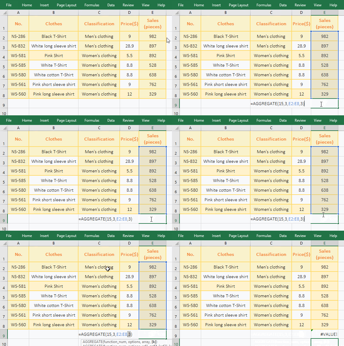
Figure 5

2. 15 means Small function in the formula =AGGREGATE(15,3,E2:E8,3), and argument Option(3) means "Ignore hidden rows, error values, nested Subtotal and Aggregate functions", argument k(3) indicates that the third minimum value is returned; when k(3) is deleted, #VALUE! is returned, indicating that the Small function cannot omit k.

III, Excel uses the Aggregate function array form to average

1. If there are turnover and price, it is required to average sales according to them. Double-click the cell E9, copy the formula =AGGREGATE(1,6,E2:E8/D2:D8) to E9, press Enter, return the value error #VALUE!; double-click the E9 again and change the formula to =AGGREGATE(14,6,E2:E8/D2:D8,2), press Enter to return to 897 that is the second maximum value of clothing sales; double-click E10, copy the formula =AVERAGE(IFERROR(E2:E8/D2:D8,FALSE)) to E10, press Ctrl + Shift + Enter to return to 750.00 that is the average of clothing sales; double-click E10 again, change FALSE to 0 in the formula, press Ctrl + Shift + Enter, return to 642.86; operation process steps, as shown in Figure 6:

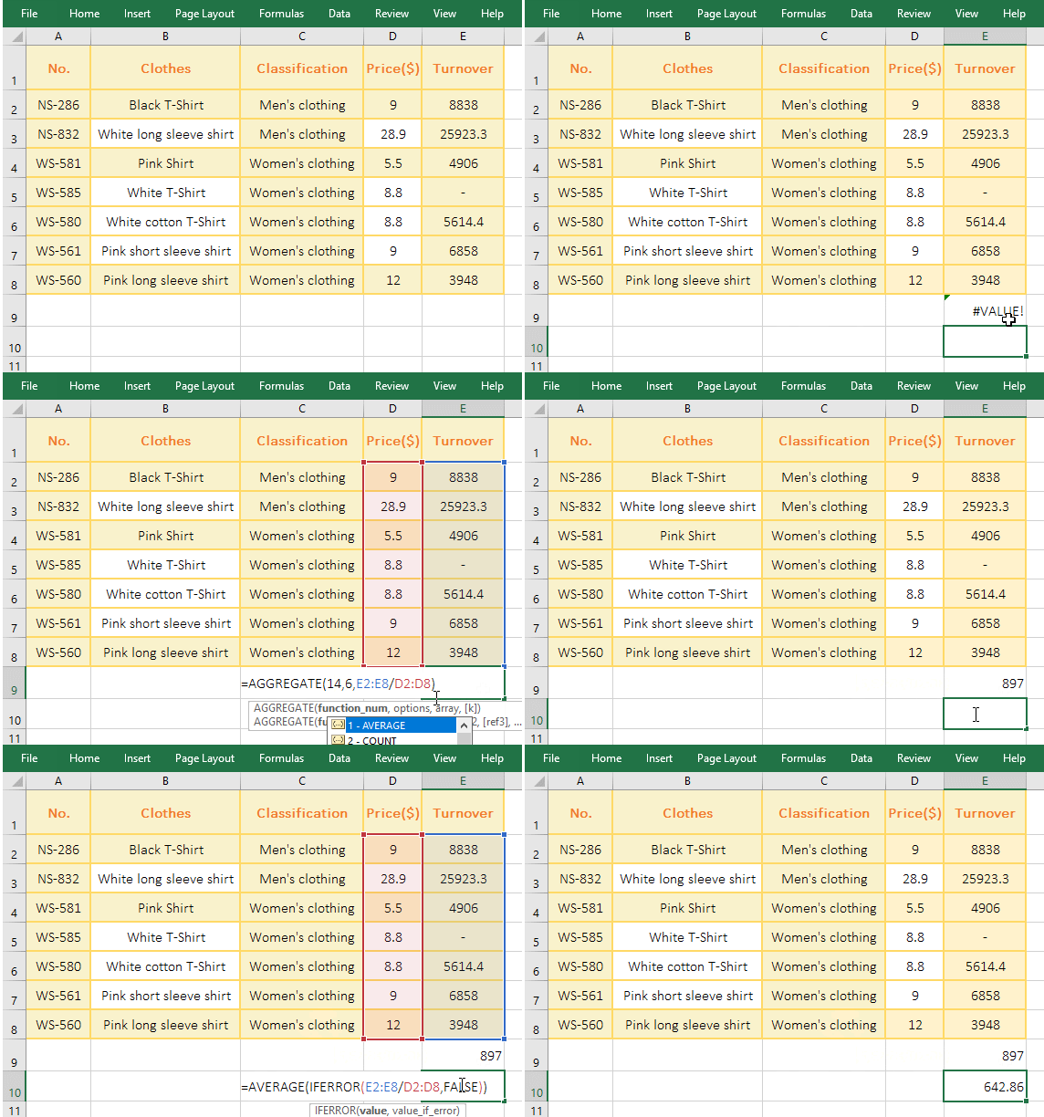
Figure 6

2. Formula description:

A. 1 means averaging, 6 means ignoring the error value in the formula =AGGREGATE(1,6,E2:E8/D2:D8), E2:E8/D2:D8 means that each element in E2:E8 divide by the element in D2:D8 that correspond to the element in E2:E8 and returns the result as an array; the original meaning of the formula is: averaging the array returned by E2:E8/D2:D8, but the Aggregate function does not support the array form of the Average function, so the return value is incorrect #VALUE!.

B. 14 means to find the maximum function Large in the formula = AGGREGATE(14,6, E2:E8/D2:D8,2), the last argument 2 means to return the second maximum; because the Aggregate function supports the array form of the Large function, so it can return the correct value. From this we can see that to use array form, you must use a function that supports arrays, that is, function numbers are 14-19.

C. IFERROR(E2:E8/D2:D8, FALSE) in the formula =AVERAGE(IFERROR(E2:E8/D2:D8, FALSE)) is used to determine each element in E2:E8 divided by the elements in D2:D8 that correspond to the elements in E2:E8, If it fails, return FALSE, otherwise return the result of division; for example, first use E2/D2, return result 982, second use E3/D3, return 897, and so on, and finally return array {982 ;897;892;FALSE;638;762;329}; then the formula becomes =AVERAGE({982;897;892;FALSE;638;762;329}), and finally averages, returns 750.00, FALSE does not participate in the average, that is, cells that contain text in E2:E8 and D2:D8 is not included.

D. After changing FALSE to 0 in the formula =AVERAGE(IFERROR(E2:E8/D2:D8,0)), the difference is that FALSE in the array that has been   returned by IFERROR (E2:E8/D2:D8,0) becomes 0, that is, {982;897;892;0;638;762;329}, then the formula becomes =AVERAGE({982;897;892;0;638;762;329}), returning the average result 642.86, 0 participates in the average, that is, the cell that contains text in E2:E8 and D2:D8 is included.