How to use Excel subtotal function(combine it with OffSet/SumProduct/If/Sum in formula)

In Excel, the SubTotal function is used to calculate subtotals. It has at least two arguments, one of which is the function number, another reference; the function number include 11 functions, and these 11 functions are set to two numbers, they are 1-11 and 101-111 respectively, 1-11 contains hidden values, 101-111 ignores hidden values, and references support up to 254.

SubTotal function can be combined with OffSet, SumProduct, If, Sum, Row and other functions; SubTotal + OffSet + SumProduct + Row is used to add products in the filter state, that is, does not contain values outside the filter; Sum + If + OffSet + SubTotal is used to return the sum of the specified conditions.

 

I, Excel SubTotal function syntax

1. Expression: SUBTOTAL(Function_Num, Ref1, [Ref2], ...)

 

2. Description:

A. Function_Num is used to specify the function to be subtotaled, there are 11 functions, each function has two serial numbers, 1-11 means to contain hidden values, and 101-111 means to ignore hidden values, as follows:

B. There must be at least one reference, and there can be at most 254 references. If a 3D reference is specified, the SUBTOTAL function will return the reference error value #REF!.

C. If there are nested subtotals in the argument ref, they will be ignored to avoid double counting; rows that are not in the filtering result are also ignored.

D. The argument Function_Num is 1-11, include the hidden value means that the value of the hidden row through the "hidden" option (ie, manually hidden); the argument Function_Num is 101-111, Ignoring the hidden value means ignoring the value of the hidden row by the "hidden" option.

E. When the argument Function_Num is 101-111, when the horizontal range is subtotaled, hiding a column does not affect the subtotal; however, hiding a row in the vertical range will affect the subtotal.

 

 

II, The use of Excel SubTotal function

(I) Sum Subtotal

1. If you want to subtotal the sum of clothing "Sales". Select the cell E9 cell, copy the formula =SUBTOTAL(9,E2:E8), and paste it in E9, press Enter, return to the result 5028; the operation steps, as shown in Figure 1:

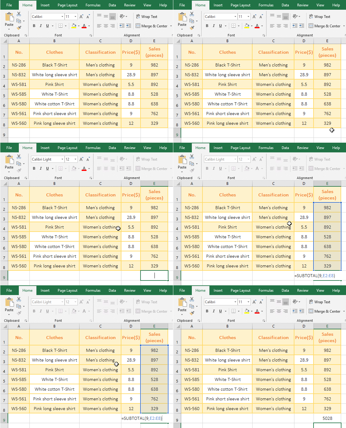
Figure 1

2. In the formula =SUBTOTAL(9,E2:E8), 9 means sum, and E2:E8 is the Sum_Range.

 

(II) Ignore nested subtotals

1. It has been subtotaled according to "Classification", and now it is subtotaled by SubTotal function. Double-click the cell D12, copy the formula =SUBTOTAL(3,D2:D11) to D12, press Enter, return to the statistical result 7; the operation steps are as shown in Figure 2:

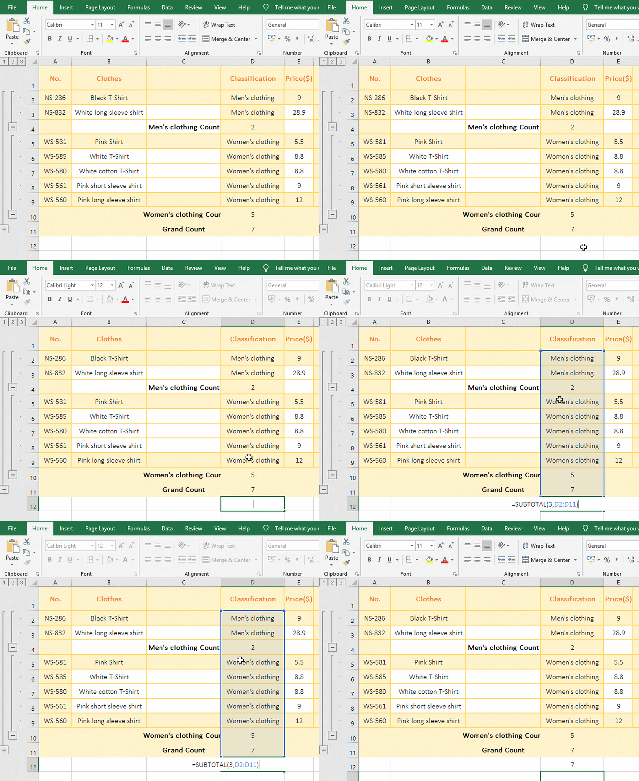
Figure 2

2. 3 means CountA function in the formula =SUBTOTAL(3,D2:D11), that is, count the number of cells that are not empty, the result is 7, indicating that there is no nested subtotal cells, because there are 10 non-empty cells from  D2 to D11 and three cells contain nested subtotals.

 

(III) Ignore rows that are not included in the screening results

1. Select the cell E9, copy the formula =SUBTOTAL(9,E2:E8) to E9, press Enter, return to the summation result 5028; select the E2:E8, select the "Data" tab, click "Filter, add the "Filter" icon to the E2 cell, click the icon, select "Number Filters" → Greater Than" in the pop-up menu, open the "Custom Auto Filter" window, and enter 600 on the "is greater than" right. Click "OK" to filter out the clothing with the sales volume greater than 600. The value in E9 automatically changes to 4171, which means that the rows not included in the screening result are ignored. The operation steps are as shown in Figure 3:

Figure 3

 

(IV) Includes hidden rows and ignore hidden rows

1. Select the cell E9, copy the formula =SUBTOTAL(2,E2:E8) to E9, press Enter, return to the count result 7 that are the numbers of cells that contain number. Select the second to fourth rows, right click the second row number 2, select "Hide" in the pop-up menu, the selected three rows are hidden, the value in E9 is still 7; double-click E9, change the 2 to 102 in the formula, press Enter, return to the statistical result 4; Operation process steps, as shown in Figure 4:

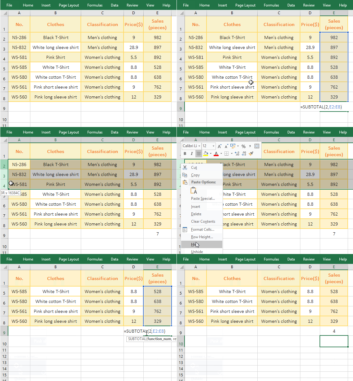
Figure 4

2. 2 represents the Count function in the formula =SUBTOTAL(2,E2:E8), when the three rows were hidden, the statistical result is still 7, indicating that the argument Function_Num is 1-11 contains hidden rows;  After 2 is changed 102 in the formula, the statistical result becomes 4, indicating that the hidden rows are ignored when the argument Function_Num is 101-111.

 

(V) The effect of hidden rows or columns on the subtotal results

1. Select the cell E10, copy the formula =SUBTOTAL(109,C2:E9) to E10, press Enter, return the sum result 15184; select the second and third row, right click the second row number 2, select "Hide" from the pop-up menu, the second and third rows were hidden; the value in E10 becomes 12311; press Ctrl + Z to unhide the rows. Right click the fourth column number D, and select "Hide" in the pop-up menu, the fourth column was hidden, the value in E10 is still 15184; the operation process steps, as shown in Figure 5:

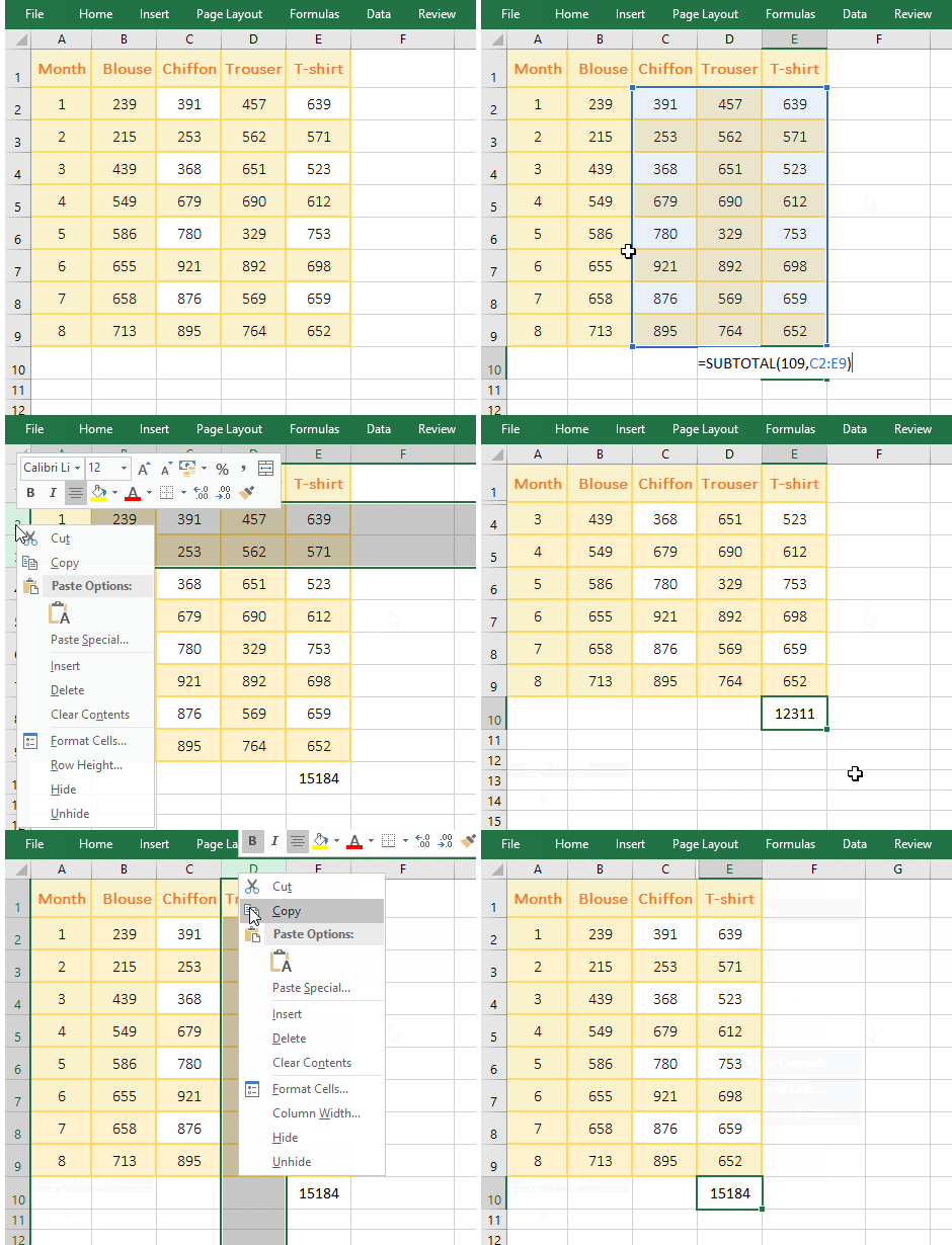
Figure 5

2. When the rows are hidden, the formula =SUBTOTAL(109,C2:E9) ignores the hidden rows; when the column is hidden, the formula =SUBTOTAL(109,C2:E9) counts the hidden column into the sum.

 

(VI) Referring to multiple ranges at the same time

1. If you require an average sales volume of any two garments (such as "Chiffon" and "T-shirt") in the clothing list. Select cell E10, copy the formula =SUBTOTAL(1,C2:C9,E2:E9) to E10, press Enter to return to 641.875; the operation steps are as shown in Figure 6:

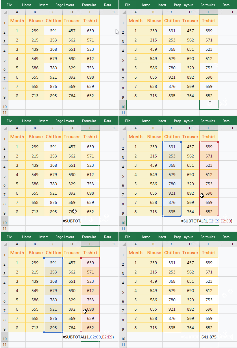
Figure 6

2. 1 means averaging in the formula =SUBTOTAL(1,C2:C9,E2:E9), C2:C9 and E2:E9 are averaging ranges.

 

 

III, Excel SubTotal function extension use case

(I) summing up to the current row

1. Double-click the cell F2, copy the formula =SUBTOTAL(9,E$2:E2) to F2, press Enter, return to the summation result 982; select the F2 again, and move the mouse to the cell fill handle on the lower right corner of F2, hold down the left button, drag down, drag to F3, sum to F2, then drag to F4, sum to D4; operation steps, as shown in Figure 7:

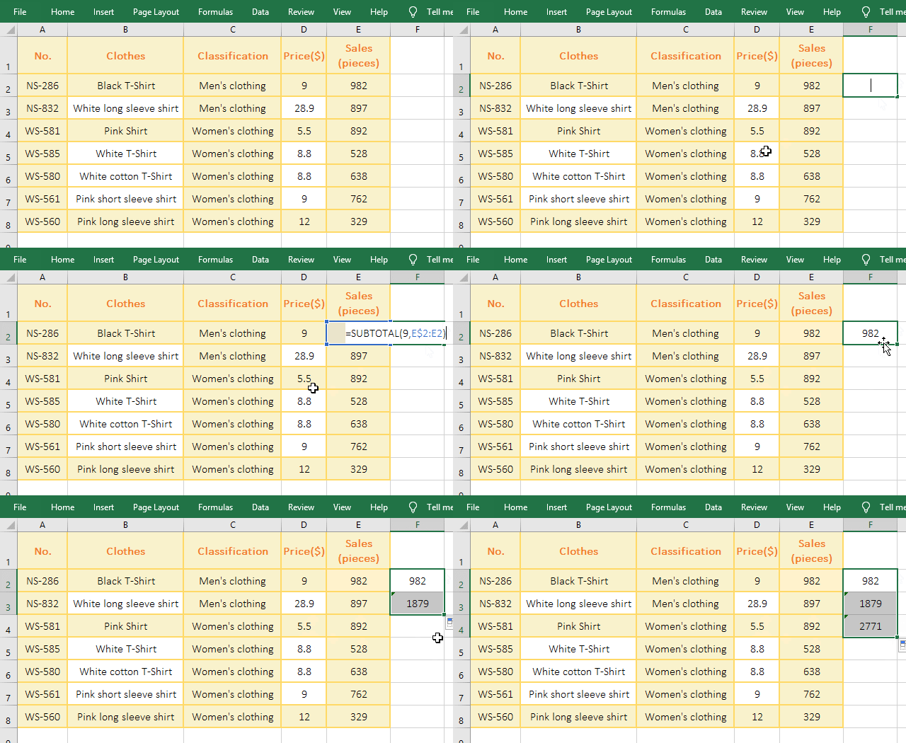
Figure 7

2. E$2:E2 in formula =SUBTOTAL(9,E$2:E2) represents reference to cell E2, and $2 represents absolute reference to the row. When dragging down, E$2 does not change, and E2 becomes E3, E4, ....

 

(II) Return the sum of the products in the filtered state with SumProduct + SumTotal + OffSet

1. If calculates the turnover in the screening state. Select cell F1, copy the formula =SUMPRODUCT((D2:D8)*(E2:E8)*SUBTOTAL(3,OFFSET(E1,ROW(1:7),)))) to F1, press Enter, and return to the result 60734.1; select E1:E8, select the "Data" tab, click "Filter", then add the "Filter" icon on E1, click the icon, select "Number Filters" → Greater Than in the pop-up menu, open the "Custom AutoFilter" window, enter 700 on the right side of "is greater than", click "OK", then filter out the clothing greater than 700, the value in F1 will become 46525.3, indicating the hidden fifth, sixth and eighth are not counted as the sum of the products; the operational steps are as shown in Figure 8:

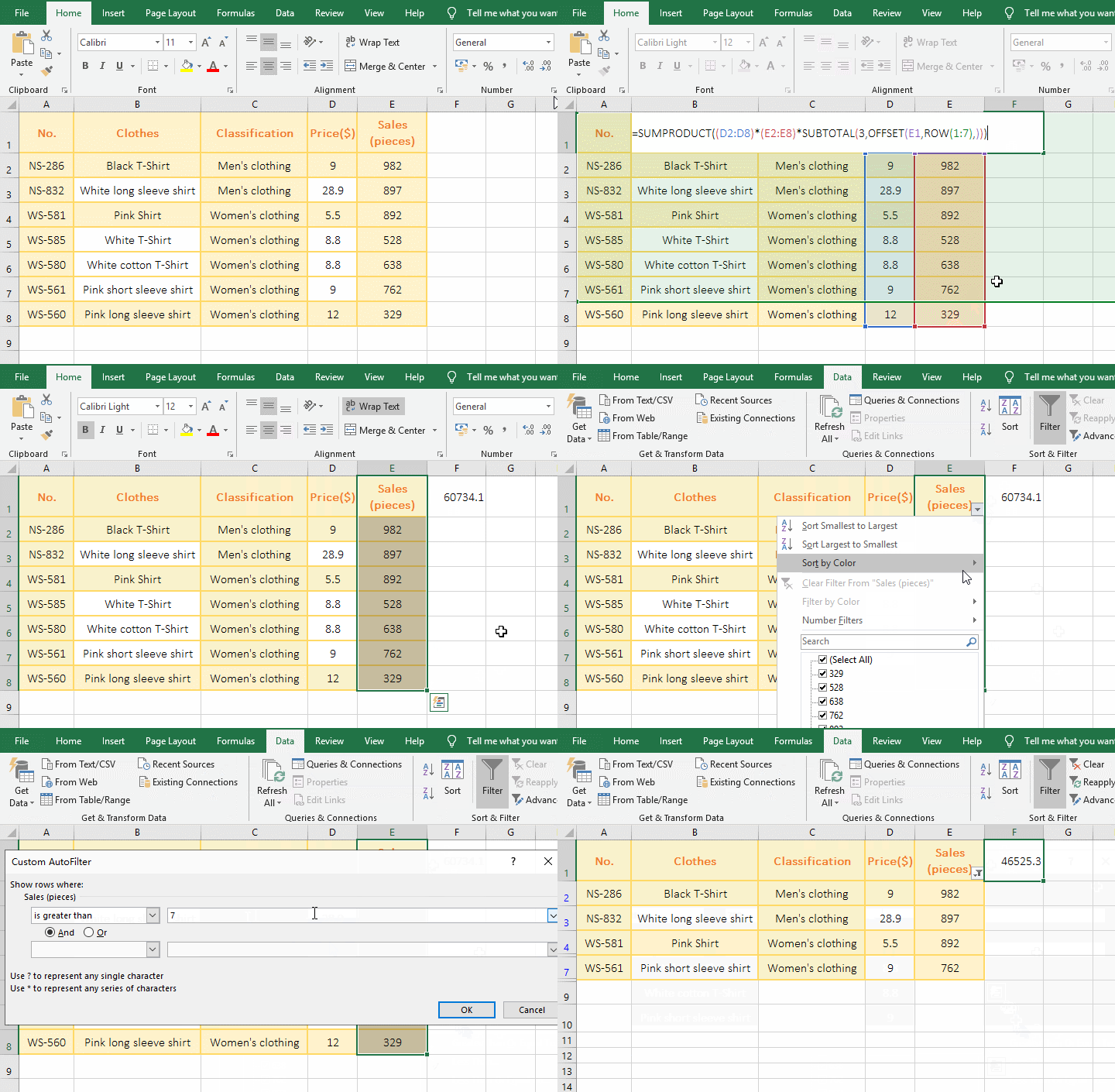
Figure 8

 

2. Formula description:

A.The formula =SUMPRODUCT((D2:D8)*(E2:E8)*SUBTOTAL(3,OFFSET(E1,ROW(1:7),)))) execution process is shown in Figure 9:

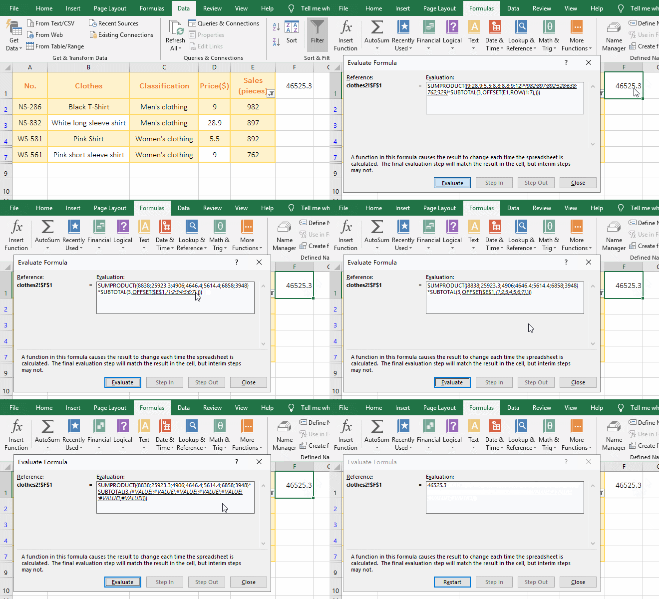
Figure 9

Formula execution process description: Select F1, hold down Alt, press M once, press V once, open the "Evaluate Formula" window, press Enter to evaluate, and press Enter once to find a value.

 

B. ROW(1:7) is used to return an array of 1 to 7, that is, {1;2;3;4;5;6;7}; then OFFSET(E1,ROW(1:7),) becomes OFFSET(E1,{1;2;3;4;5;6;7},), when executed, starting in E1, take 1 from the array as the argument Rows for the first time, because the Offset function omits the argument Cols, return the height and width of the cell, thus returning the value of cell E2 in the next row of E1; take 2 from the array as the argument Rows for the second time, return the value of cell E3 in the second row of E1, and so on; and finally return the array {#VALUE!;#VALUE!;#VALUE!;#VALUE!;#VALUE!;#VALUE!;#VALUE!}, #VALUE! represents the value in E2:E7, which can be used with the formula =SUM(N(OFFSET(E1,ROW(1:7),))) Verify (press Ctrl + Shift + Enter after entering the formula), as shown in Figure 10:

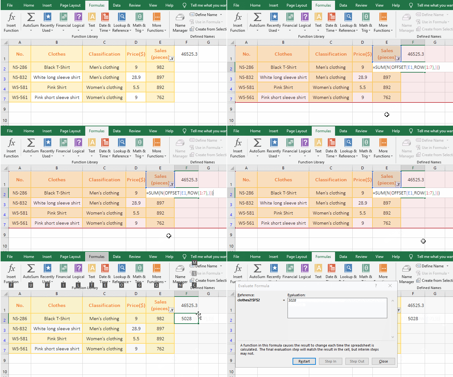
Figure 10

 

C. Then SUBTOTAL(3, OFFSET(E1, ROW(1:7),)) becomes SUBTOTAL(3,{#VALUE!;#VALUE!;#VALUE!;#VALUE!;#VALUE!;#VALUE! ;#VALUE!}), when executed, each value is taken out of the array in turn, if it is hidden (ie not filtered), it returns 0, otherwise it returns 1, and finally returns {1;1;1;0;0;1;0}, it corresponds to the fifth, sixth, and eighth rows are hidden. Note that the range here is E2:E8, so E2 is the second row, so the first element of the array is 1.

D. D2:D8 returns the value in D2 to D8 as an array, E2: E8 returns the value in E2 to E8 as an array, then multiplies the corresponding elements of the two arrays, and finally returns the array {8838;25923.3;4906;4646.4;5614.4;6858;3948}.

E. Then the formula becomes =SUMPRODUCT({8838;25923.3;4906;4646.4;5614.4;6858;3948}*{0;0;1;0;1;1;1}), and then the two arrays correspond to the elements Multiply, then calculate the sum of each product.

 

 

(III) Use the Sum + If + SubTotal + OffSet function to calculate conditionally the sum that don't  include hidden values.

1. If the sum of sales of "Men's clothing" is required. Double-click the cell E9, copy the formula =SUM(IF(C2:C8="Men's clothing", SUBTOTAL(109,OFFSET(E1,ROW(1:7),))))) to E9, press Ctrl + Shift + Enter, return the summation result 1879; right click the third row number 3, select "hidden" in the pop-up menu, then the third row (Classification as Men's clothing) is hidden, the value in E9 will change to 982, indicating the hidden row don't add to summation; the operation process steps are as shown in Figure 11:

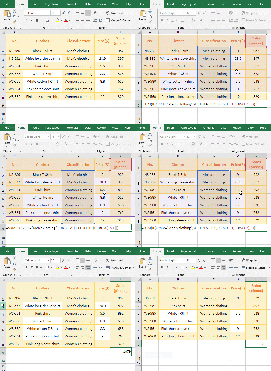
Figure 11

 

2. The formula description(to hide the third row as an example): =SUM(IF(C2:C8="Men's clothing", SUBTOTAL(109,OFFSET(E1,ROW(1:7),)))))

A. OFFSET(E1,ROW(1:7),)) has been analyzed in the above example, and finally returns {#VALUE!;#VALUE!;#VALUE!;#VALUE!;#VALUE!;#VALUE!;#VALUE!}.

B. SUBTOTAL(109,OFFSET(E1,ROW(1:7),)) becomes SUBTOTAL(109,{#VALUE!;#VALUE!;#VALUE!;#VALUE!;#VALUE!;#VALUE!;#VALUE!}), then, return 0 if the value in the array is hidden, otherwise return a specific value, and finally return {982;0;892;528;638;762;329}.

C. C2:C8="mMen's clothing" is the condition of If, meaning: if the text in C2 to C8 is equal to "Men's clothing", return True, otherwise return False; for example, the text in C2 is "Men's clothing", so return True, the text in C3 is "Women's clothing", so return False; finally return the array {TRUE;TRUE;FALSE;FALSE;FALSE;FALSE;FALSE}.

D. Then the formula becomes =SUM(IF({TRUE;TRUE;FALSE;FALSE;FALSE;FALSE;FALSE},{982;0;892;528;638;762;329})), then the corresponding elements in the two arrays are multiplied (when True is converted to 1 and FALSe is converted to 0), the formula becomes =SUM({982;0;FALSE;FALSE;FALSE;FALSE;FALSE}), and finally returns 982.

Hint: If + SubTotal combination cann't be writed: =SubTotal(109,If(C2:C8="Men's clothing"), C2:C8,)).