Excel pivot table percentage of grand total(parent row or column), difference from, running total in

 The Show Value As in pivot table is primarily used to subtotal percentages in excel. It includes the percentage of grand total; the percentage of row and column total; the percentage of parent row total, parent column total and parent total; difference from and the percentage of difference from; running total in and the percentage of running total in; where the abstract is the percentage of parent row total, parent column total and parent total.

The percentage of the parent row total is often used to subtotal the percentage of sales in different regions of the product in all regions; the percentage of the parent column total is often used to subtotal the monthly sales as a percentage of the total sales, it needs to first merge the data for each month into the pivot table with the multiple consolidation ranges; the percentage of parent total is more flexible, it can specify a field as a parent field, and then calculate the percentage of the fields of its child and subfields of its child.

I, The percentage of grand total and an item(Show Value As in pivot table)

(I) Excel pivot table percentage of grand total(% of grand total)

1. If you want to calculate the percentage of grand total of "Payable salary". Move your mouse over the "Payable salary($)" field, hold down the left button, drag it to the "∑ Value" list box, double-click the cell C3, open the "Value Field Settings" dialog, and change the name to "% of grand total", click "OK"; right click C4, select "Show Value As → % of Grand Total" in order in the pop-up menu, then calculate the percentage of each employee and department's salary respectively to the total salary; the operation process steps, see screenshot in Figure 1:

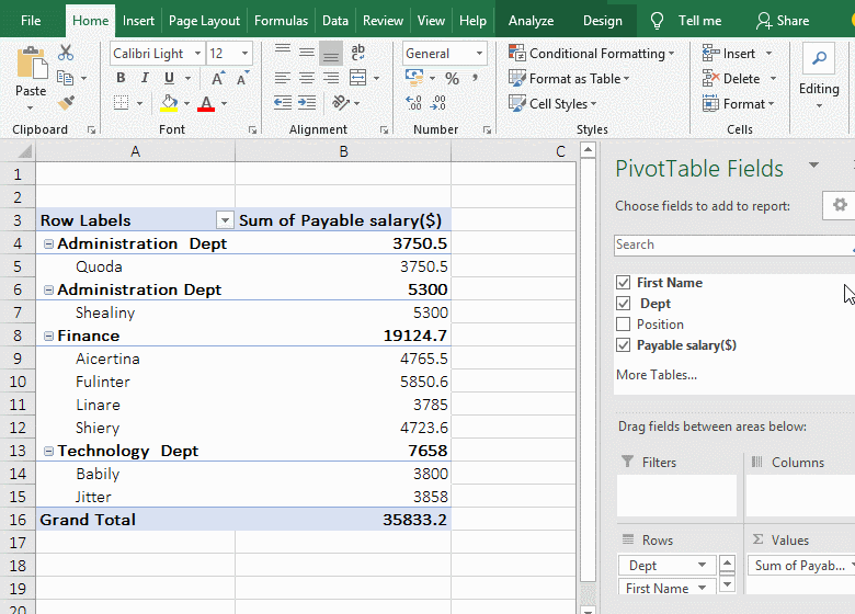
Figure 1

2. The calculation method is: the percentage of grand total = the value of an item / the grand total, for example, the percentage of grand total of the salary of "Finance" is calculated, which is equal to 19124.7/35833.2 = 53.37%.

(II) Excel pivot table percentage of an item(% of ...)

1. If you want to calculate the salary of other departments as a percentage of the finance department's salary. Then drag a "Payable salary($)" field to the "∑ Value" list box, double-click D4, open the "Value Field Settings" dialog, change the name to "% of ..."; right click D4, select "Show Value As → % of ..." in the pop-up menu, open the "Show Value As(% of ...)" dialog, select "Dept" for "Basic Field", "Finance" for "Basic Item", and click "OK", then calculate the percentage of salary of other departments(Administration and Technology Dept) to the salary of "Finance"; the operational steps, as shown in Figure 2:

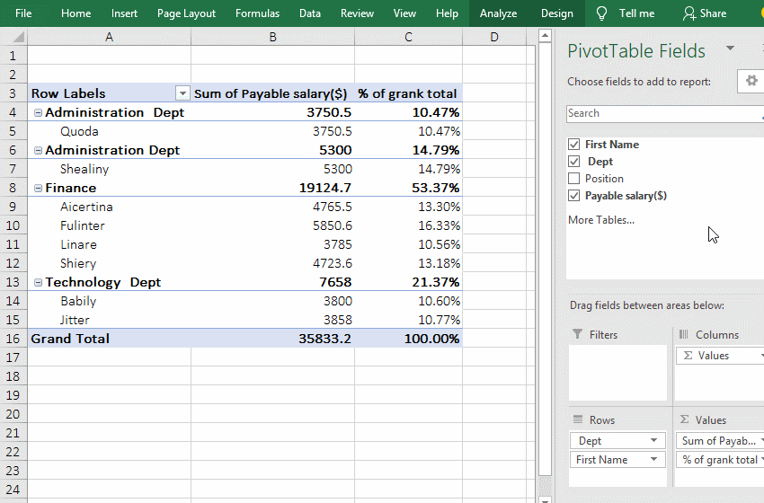
Figure 2

2. The calculation method is: % of ... = the value of ... / the value of base item. For example, the Finance's salary is 100%, because it is the basic item, the salary of "Administration Dept" is 19.61%, it is calculated by the total salary of "Administration Dept" compared to the total salary of the "Finance"(ie 3750.5/19124.7), the 40.04% of the "Technology Dept" should be calculated this way.

The difference between % of grand total and % of ...: the former uses one item compared to the grand total, such as the total salary of the "Finance"(or the salary of an employee) compared to the total salary; the latter uses one item compared to the basic item (ie, the designated item), for example, the total salary of the "Administration Dept" is compared with the total salary of the designated "Finance" in the demonstration.

II, The percentage of column total and row total(Excel PivotTable Show Value As)

(I) The percentage of column total(% of column total)

1. If you want to subtotal the percentage of sales of all types of clothing and each piece of clothing accounted for the total sales of all clothing. As shown in the above example, drag a "Sales" field to the "∑ Value" list box, double-click C3, change the name to "% of column total" in the open dialog, and click "OK"; right-click C4, select "Show Value As → % of column total" in the pop-up menu, then subtotal the percentage that meets the criteria; the operational steps, see screenshot in Figure 3:

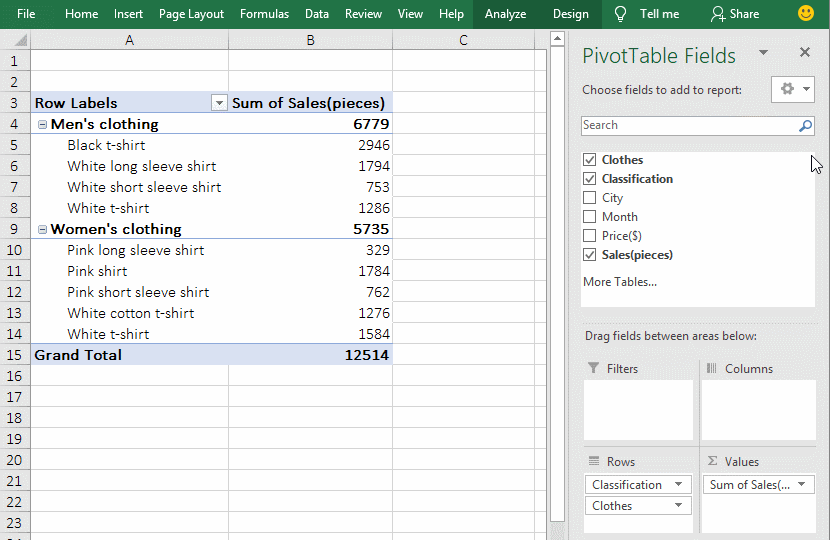
Figure 3

2. The calculation method is: % of column total = the value of an item / the value of the column total. For example, to calculate the percentage of column total of the "Black t-shirt", it is equal to 2946/12514.

(II) The percentage of row total(% of row total)

The percentage of row total is only calculated in one row in a column, that is, the value of one cell is compared with itself, the result is 100%. It cannot subtotal each column in a row before calculating, so the result is not the percentage of the subtotal of each column in a row; if you want to achieve this, you need to use "multiple consolidation ranges" to generate the PivotTable. For details, please refer to the "% of parent column total".

III, The percentage of parent row, parent column and parent total(Excel PivotTable Show Value As)

(I) The percentage of the parent row total(% of parent row total)

1. If you want to subtotal the percentage of parent row total of sales of clothes in the region. Move the mouse to the field "Sales(pieces)", hold down the left button and drag it to the "∑ Value" list box, double-click the cell C3, in the open dialog, change the name to "% of parent row total", click "OK"; right click C3, select "Show Value As → % of parent row total" in the pop-up menu, then subtotal the percentage of parent row total of sales of 
each piece of clothing and each city; the operation process steps, as shown in Figure 4:

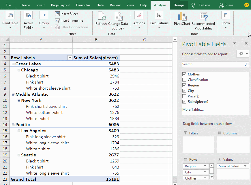
Figure 4

2. Calculation method:

A. The % of parent row total = the value of an item / the value of the parent row. "The value of the parent row" has different meanings for different levels of row, take the row in the demo, it is divided into four categories, one is the row where each piece of clothing is located, the second is the row where the clothing sales in the city is located, the third category is the row where "Region" is located, the fourth category is the row where "Grand Total" is located; the second category is the parent row of the first category(eg "Chicago" is the parent row of "Black t-shirt"), the third category is the parent row of the second category (eg "Great Lakes" is the parent row of "Chicago"), and the fourth category is the parent row of the third category(such as "Grand Total" is the parent row of "Great Lakes").

B. Specific calculation examples. The percentage of the parent row total of "Black t-shirt" = B6(2946)/B5(5483), the percentage of the parent row of "Chicago" = B5(5483)/B4(5483), the percentage of the parent row total of "Great Lakes" = B4(5483)/B23(15191). Hint: B in the calculation formula is actually C, in order to facilitate the viewing of specific values, B is used instead of C, the same below.

(II) The percentage of the parent column total(% of parent column total)

1. There is a pivot table whose clothing sales are from April to June, it asks to calculate the percentage of the parent column total. Right-click any cell in the data region(such as C5), select "Show Value As → % of the parent column total" in the pop-up menu, and calculate the sales percentage of each garment in April to June; the steps are as shown in Figure 5:

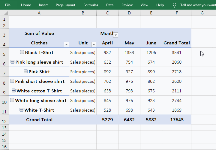
Figure 5

Tip: The "clothing sales from April to June in pivot table" in the demo is generated by multiple consolidation ranges for the three clothing sales tables in April, May, and June. Each table has the same structure and is composed of the field "Clothes and Sales", specifically how to merge, please see the article "Combine multiple excel sheets into one pivot table with multiple consolidation ranges in excel". The columns(April, May, and June) in the pivot table are the sales in the months in the original table.

2. Calculation method:

A. The % of the parent column total = the value of an item / the value of the parent column. For example, the sales 982 in April(that is, the value of C5) of "Black T-Shirt" is the value of a certain item, and the "Grand Total" of the Black T-Shirt" that is 3541(that is, the value in F5) is "the value of the parent column".

B. Calculation examples. The percentage of parent culumn total of sales of the "Black T-Shirt" in April = C5/F5, which is 982/3541 = 27.73%; the percentage of parent column total of salse of the "white shirt" in May = D5/F5, ie 1353/3541 = 38.21%.

(III) The percentage of parent total(% of parent total)

1. Take the percentage of parent total of clothing sales in the regions as an example. Drag the "Sales" fields to the "∑ Value" list box, double-click cell C3, open the "Value Fiesd Settings" dialog, change the "Custom Name" to "% of parent total", click "OK"; right-click the cell C4, Select "Shows Value As → % of parent total" in the pop-up menu, open the "Show Value As(% of parent total)" dialog, select "Region" for "Basic Field", click "OK" or press Enter, then total the percentage of paretn total of salse of each clothing and city; the operational steps, see screenshot in Figure 6:

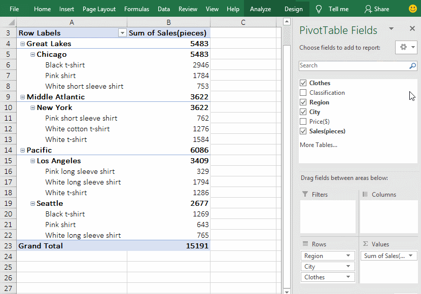
Figure 6

2. Calculation method:

A. The percentage of parent total = value of an item / value of the specified "basic field". "Value of an item" is a child, and the value of the specified "basic field" is a parent; for example, each piece of clothing(such as "Black t-shirt") and city (such as "Chicago") are children in the presentation, region( Such as "Great Lakes") as a parent.

B. The specific calculation examples. The percentage of parent total of the "White shirt" in A18 = B18(1286)/B14(6086), the percentage of parent total of "Los Angeles" = B15(3409)/B14(6086).

IV, The difference from and percentage difference from(Excel PivotTable Show Value As)

(I) Difference from

1. If you calculate the difference from region of the sales of clothing as an example. Drag the "Sales" fields to the "∑ Value" list box, double-click cell C3, open the "Value Field Settings" dialog, change the "Custom Name" to "Difference from region", click "OK"; right-click C3, select "Show Value As → Difference From" in the pop-up menu, open "Show Value As(Difference from region)" dialog, select "Region" for "Basic Field" and "Pacific" for "Basic Item", Click "OK" to calculate the difference between the sales of clothing in "Great Lakes" and the sales in "Pacific" -603; the operation steps are as shown in Figure 7:

Figure 7

2. Calculation method:

A. Difference from = value of an item - specify the value of the "Basic Field". For example, calculate the difference from region, the "Pacific" is the basic field, and other regions(such as "Great Lakes or Middle Atlantic") are certain items in the demonstration.

B. Calculation examples. The difference of sales of clothes between in "Great Lakes and Pacific" = B4(5483)- B14(6086)= -603; The difference of sales of clothes between in "Seattle" and "Los Angeles" = B19(2677)- B15(3409)= -732.

(II) The percentage of difference from

1. Take "the difference from region" to "the percentage of difference from region" above as an example. Double-click cell C3, open the "Value Field Setting" dialog, change the "Custom Name" to "% Difference from region"; right-click C3 where "Difference from region" is located, select "Show Value As → % Difference From" in the pop-up menu, open the "Show Value As(% Difference from region)" dialog, select "Region" for "Base Field", select "Pacific" for "Basic Item", click "OK", then calculate the percentage(-9.91%) of difference between the sales of clothing in "Great Lakes" and the sales in "Pacific"; the operation process steps are as shown in Figure 8:

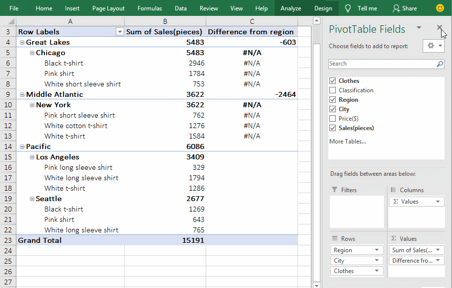
Figure 8

2. Calculation method:

% difference from = (value of an item - specify the value of "Basic Field") / Specify the value of "Basic Field". For example, calculate the percentage of difference in sales of clothing between "Great Lakes" and "Pacific", calculated as: (B4(5483)- B14(6086))/ B14(6086)= -603/6086 = -9.91%.

V, Running total in and the percentage of running total in(Excel PivotTable Show Value As)

(I) Running total in

1. If the sales of clothing in the city are subtotalled as an example. Drag the "Sales" fields to the "∑ Value" list box, and rename the text in C3 to "Running total in city", and right click C3, select "Show Value As → Running total in" in the pop-up menu, select "City" for "Basic Field" in the dialog that has been opened, click "OK" to return the subtotals with the "City" as the basic field; the operation process steps, see screenshot in Figure 9:

Figure 9

2. As you can see from the demo, when the "city" is the basic field and only aggregated to the city, the "Regions" are not subtotalled, and the subtotal in cities is to accumulate sales per city; For example, the subtotal result of "Seattle" is 6086, which is the sales in Los Angeles + in Seattle. When "Region" is used as the basic field, the "Region" and its children are subtotalled, for example, the sales in Great Lakes, Middle Atlantic, Pacific and cities in this three regions are subtotalled; but it will not subtotal the superior fields of the "Region", For example, there is no subtotal "Grand Total". 

(II) The percentage of running total in

1. To change the "Running total in city" above to "% Running total in city" as an example. Change "Running total in city" in C3 to "% Running total in city"; right-click C3, select "Show Value As" → % Running total in" in the pop-up menu, select "City" for "Basic Field" in the dialog that has been opened, click "OK", calculate the percentage with "City" as the basic field; see screenshot in Figure 10:

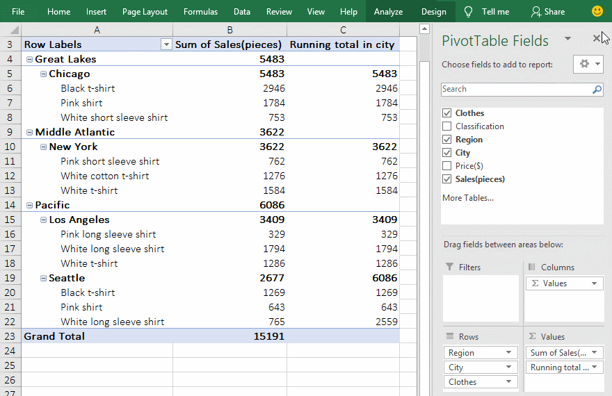
Figure 10

2. It can be seen from the demonstration that when "City" is used as the basic field, the "% Running total in Los Angeles" is calculated as =B15/(B15+B19) , ie 3409/(3409 + 2677) = 56.01%, the "% Running total in Seattle" is calculated as =(B15+B19)/(B15+B19), ie (3409 + 2677)/(3409 + 2677) = 100%; the same calculation method with "Region" as the basic field.