How to filter in excel(16 examples, with number,text,color,duplicates,shortcut,multiple criteria)

There are two ways to filter in Excel, one is to use the "Filter" in the right button menu of mouse to quickly filter, and the other is to use the options in the "Filter" drop-down menu to filter. Excel filter is divided into five categories, namely number filter, text filter, cell color filter, font color filter and cell icon filter.

In addition to filtering by one condition, it can also filter by two conditions, and can also filter multiple columns at the same time. There are also two combinations of conditions, one bases on option and the other uses wildcard. The filtered operation can be done with both the mouse and shortcut.

I, How to filter in excel

(I) Filter number

1. How to filter out duplicates in excel(Filter by Selected Cell's Value)

Suppose you want to filter all students whose score is 684. Right-click one of the cells with a score of 684(such as B2), select "Filter" from the pop-up menu, and select "Filter by Selected Cell's Value" in the expanded sub-option, and filter all students whose scores are 684 points; steps of the operation process, as shown in Figure 1:

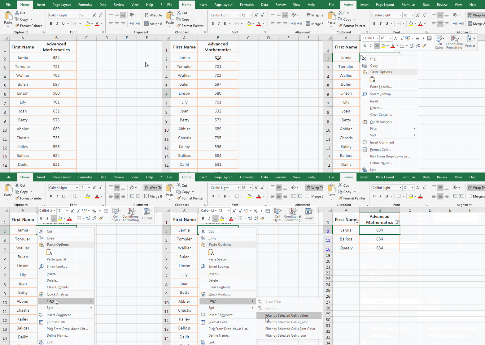
Figure 1

2. Filter top 3, 5, and 10 items

A. If you want to filter the top 3, 5, and 10 of the "Advanced Mathematics" scores. Click column number B in the second column, select column B, select the "Data" tab, click the "Filter" icon, then a filter icon in the lower right corner of the cell B1, click the icon, Select "Number Filters" → Top 10 in the pop-up menu, open the "Top 10 AutoFilter" dialog, click "OK" to automatically filter out the top 10; in the same way, open the "Top 10 AutoFilter" dialog and change 10 to 3, click "OK", the first 3 are automatically selected; the first 5 filters are the same method; the operation steps are as shown in Figure 2:

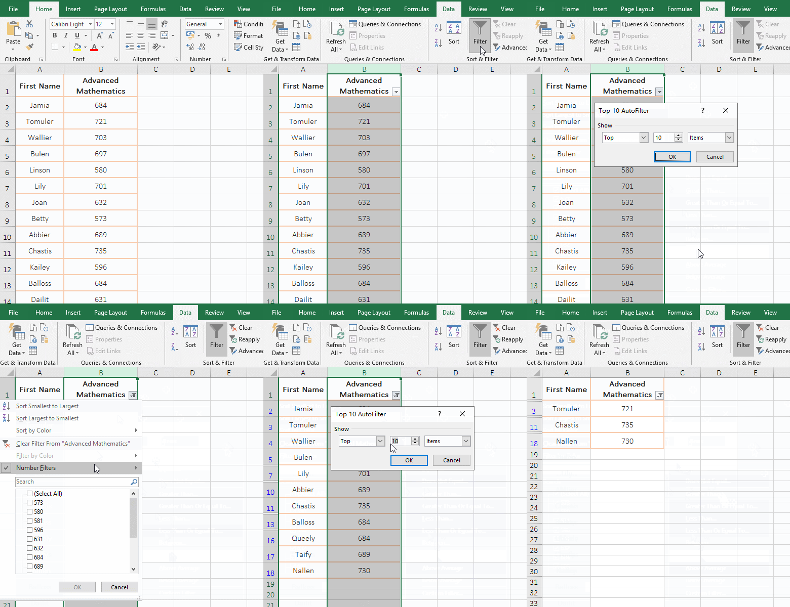
Figure 2

B. In addition to filtering the first few items, you can also filter the last few items, in the "Top 10 AutoFilter" dialog, select "Maximum" as "Minimum"; the filter value can also be "Percentage", in the "Top 10 AutoFilter" dialog, select "Item" as "Percent".

3. Filter all items above or below the average

Click column B in the second column, select column B, select the "Data" tab, click the "Filter" icon, the filter icon appears in the lower right corner of B1; click the icon, select "Number Filters" → Above the average in the pop-up menu, all the students' names and grades above the average score are automatically filtered; the same method is used to filter all students below the average score; the operation steps are as shown in Figure 3:

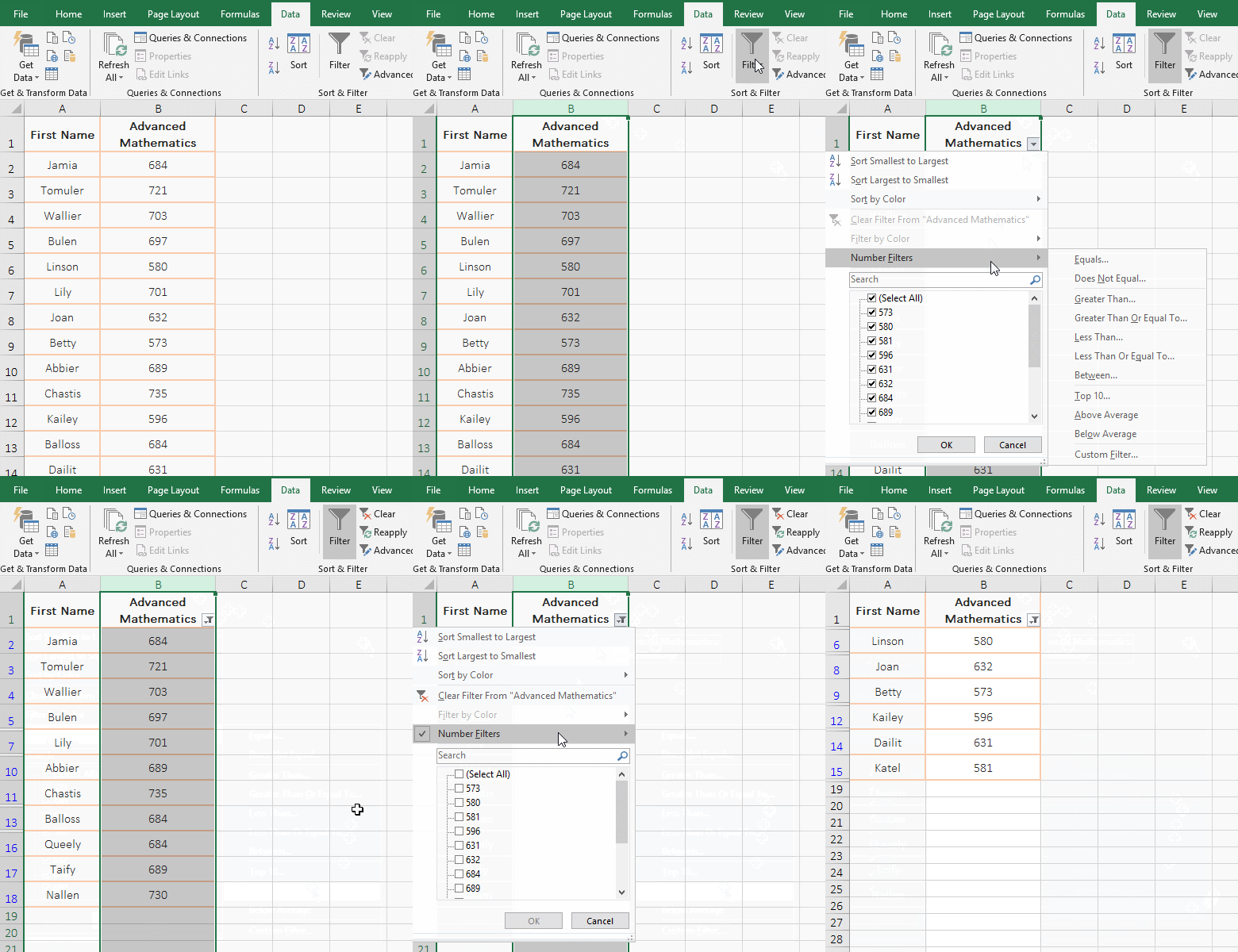
Figure 3

4. Filter by criteria

A. Filter by a criterion. If you want to filter the scores above 700 points. Select column B, select the "Data" tab, click the "Filter" icon, add a filter icon in the lower right corner of B1, click the icon, select "Number Filters" → Greater Than in the pop-up menu, open "Custom AutoFilter" dialog, enter 700 on the right side of "is greater than", press Enter or click "OK" to filter out all students with more than 700 points; the operation steps are as shown in Figure 4:

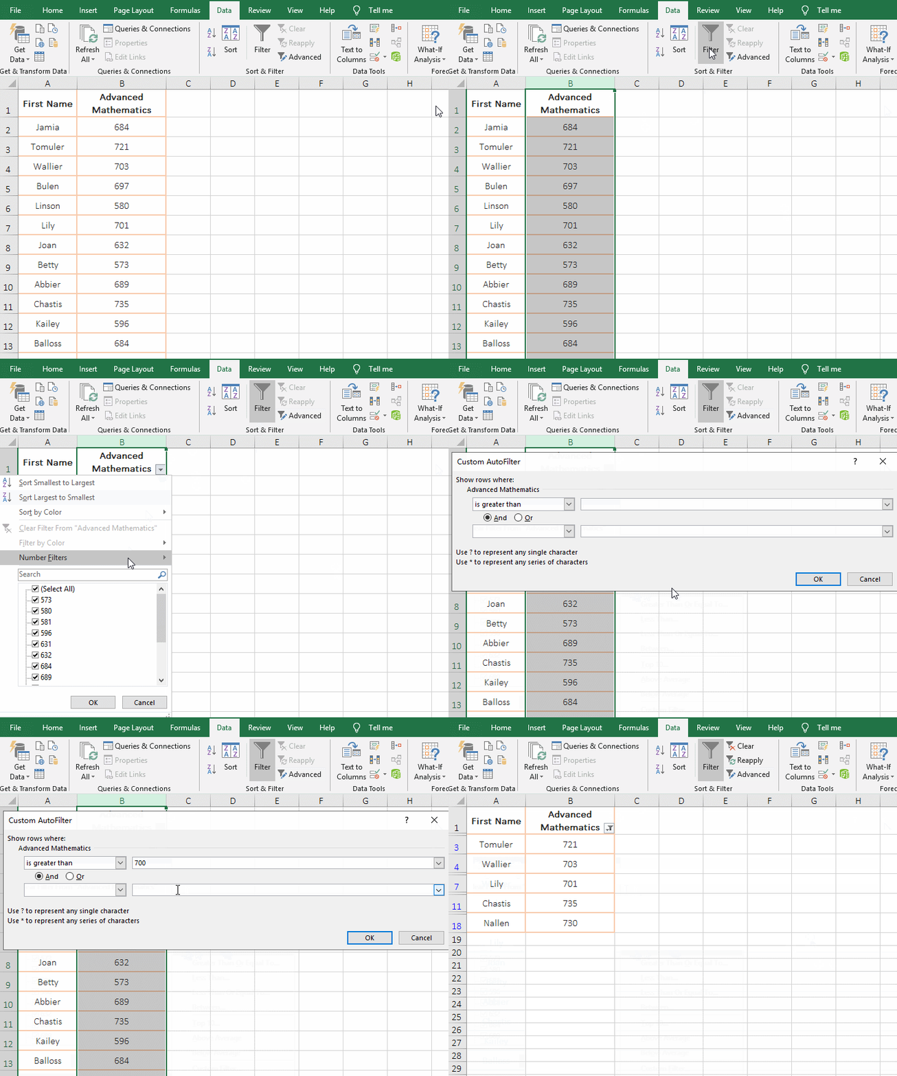
Figure 4

B. Filter by double criteria. If you want to filter the scores of "Advanced Mathematics" between 600 and 700 points. Select column B, add a filter icon like filter by a criterion, click the icon, select "Number Filter" → less Than or Equal to in the pop-up menu, open the "Custom AutoFilter" dialog, enter 700 on the right side of the first criteria, enter 60 on the right side of the second criteria, press Enter to filter out all the students who meet the criteria; the process steps, see screenshot in Figure 5:

Figure 5

In the demonstration, since two criteria are to be met, "AND" is selected between the first and second criteria; if only two criteria are required to satisfy one criteria, "OR" should be selected.

(II) Excel text filter

1. Precision filter

A. If you want to filter all employees of the "Finance Department". Click the column B of the second column, select the second column, select the "Data" tab, click the "Filter" icon, then add a filter icon in the lower right corner of B1, click the icon, and then select "Text Filters" → Equal in the pop-up menu, open the "Custom AutoFilter" dialog, enter "finance" on the right side of "equals", press Enter to automatically filter out all the finance department employees; the operation process steps are as shown in Figure 6:

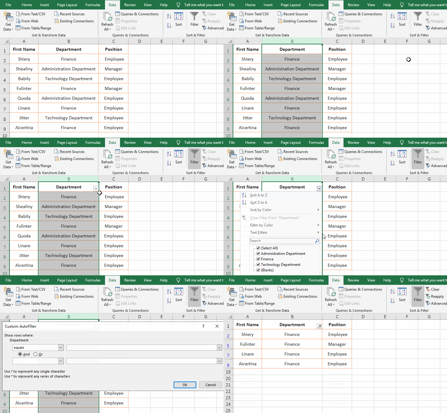
Figure 6

B. If you select "Not equal to", it means filtering all employees except "Finance Department".

2. Fuzzy filter

A. If you want to filter all clothes that start with "White" and contains "long". Select column B, add a filter icon to column B like precision filtering, click the icon, select "Text Filters" → Begins With from the pop-up menu, open the "Custom AutoFilte" dialog, copy "White" to the textbox on the right of the "begins with" , click the drop-down list box to the left of the second criteria, select "contains", then enter "long" on the right, there are "AND" and "OR" between the two criteria, keep the default selection "AND", press Enter, select all the garments that meet the two criteria; the operation steps are as shown in Figure 7:

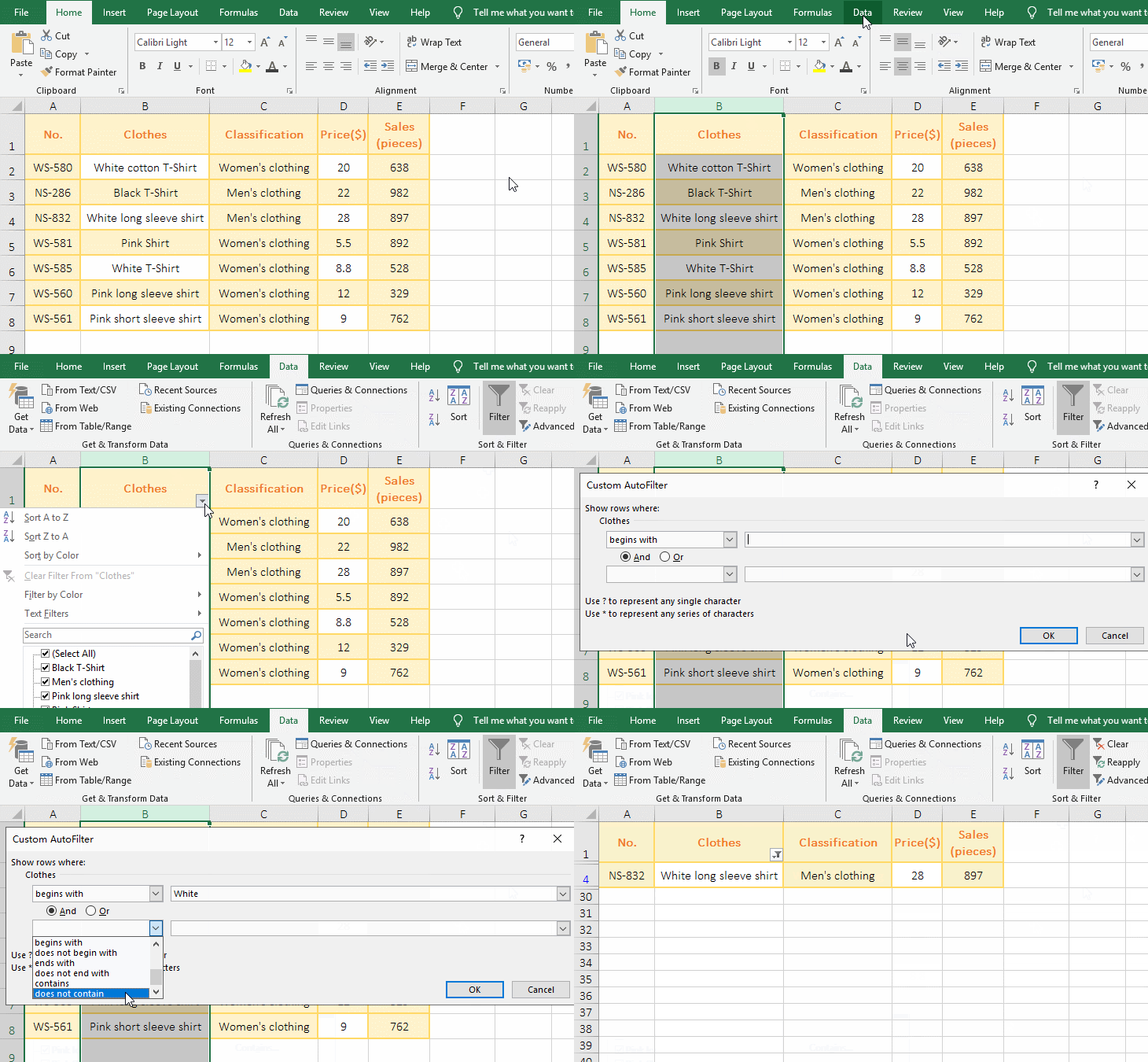
Figure 7

B. If you want to filter the clothes ending with any character, select "Ends With" in the menu of "Text Filters" to expand, and then enter the specified characters in the open dialog.

(III) Filter by color

1. Filter by cell color; select column A, click the "Filter" icon under the "Data" tab, add a filter icon to column A, click the icon, and select "Filter by Color" → "Filter by cell color"  → "Light orange" in the pop-up menu, filters out the clothing whose background is the color.

2. Filter by font color. Click the Filter icon again, the filter icon in column A is canceled, select column C, click the filter icon again, add a filter icon in column C, click the icon, and select "Filter by Color" → "Filter by font color" → "Green" from the pop-up menu, then filter out all the clothes whose names are green; the operation steps are as shown in Figure 8:

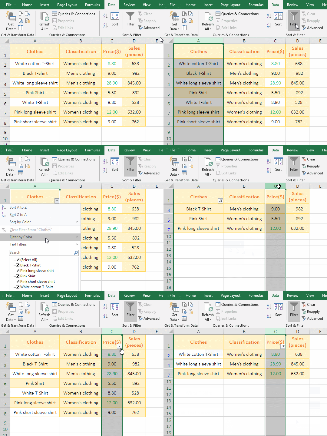
Figure 8

Hint: The text in column C has tow colors(green black), only green is available for selection. If you want to filter all clothing with black text, select "Automatic".

(IV) Filter by cell icon

If only the price marked with the golden star icon is selected. Select column C, click the "Filter" icon under the "Data" tab, add the icon to column C, click this icon, select "Filter by color" → "Filter by Cell Icon" →  "golden star" in the pop-up menu, it automatically filters out a price marked with the icon; the operation process steps, see screenshot in Figure 9:

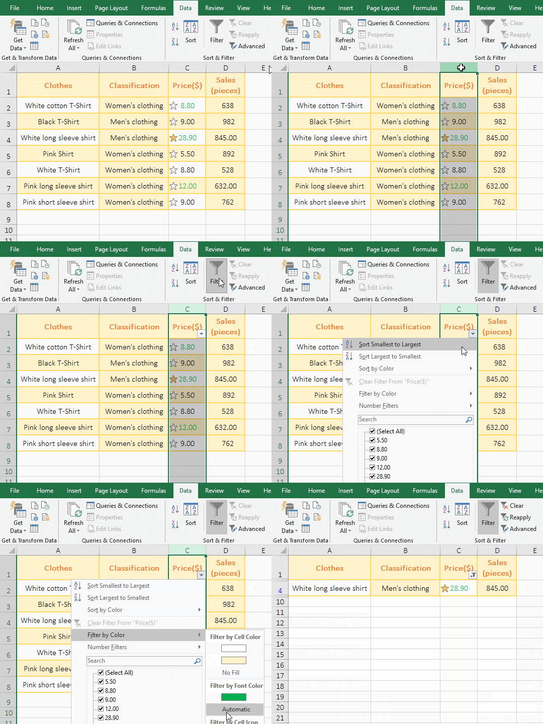
Figure 9

II, How to use search filter in excel

(I) How to search multiple items in excel filter

1. If you want to filter any one or several scores to be specified in the "Advanced Mathematics" scores. Select column B, select the "Data" tab, click the "Filter" icon, add this icon to column B, click it, click "Select All" to deselect all in the pop-up menu, then click 631 to check it, click "OK" to filter out all the students with 631 points; click the "Filter" icon in column B again, and then check 584 and 689 in the pop-up menu to filter the selected All students with the scores; steps of the operation process, see screenshot in Figure 10:

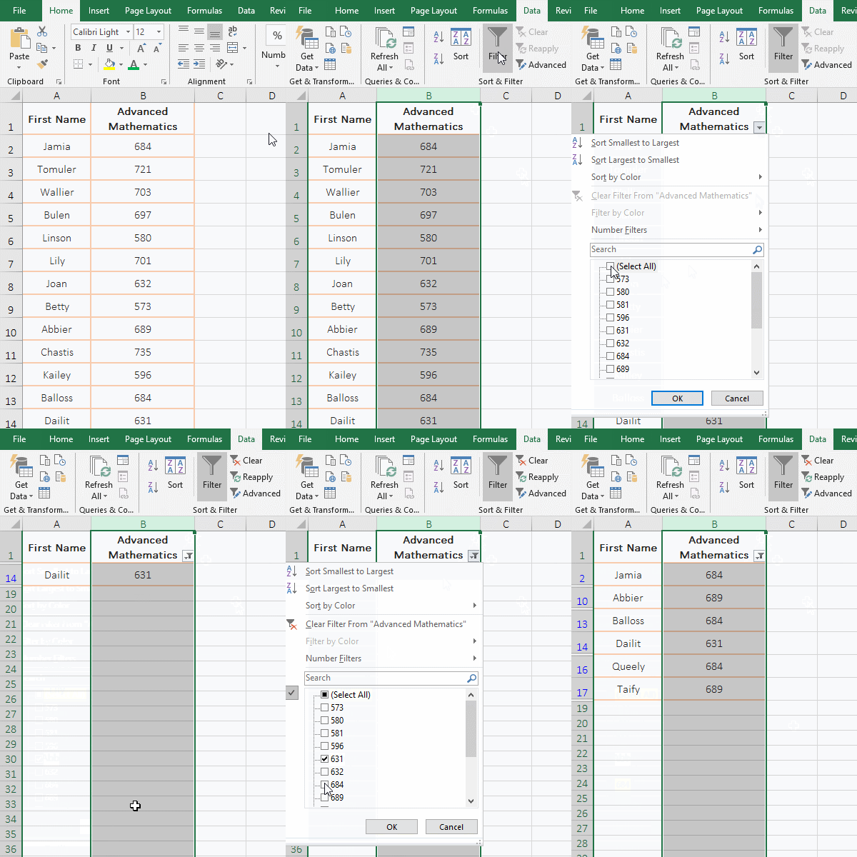
Figure 10

2. If the column to be filtered is text, you can also use this method to filter.

(II) How to filter by inputting text to be searched

1. Filter clothes that start with the word "white". Select column A, add a "filter" icon to column A, click on it, in the pop-up menu, enter "white*" or "white" in the search input box, press enter "OK", then filter out all the clothes that start with "white"; * is a wildcard, indicating any one or more characters, "white*" means beginning with "white", there can be any one or more characters after "white".

2. Filter clothes containing the word "long". Click the "Filter" icon in the lower right corner of A1 again, in the pop-up menu, enter "*long*" and press "Enter" to filter out all the clothes containing "long".

3. Filter clothes with only ten characters. Then click the "Filter" icon of A1, in the pop-up menu, enter ten question marks ??????????, press Enter to "OK", then filter out only ten characters clothes; operation steps, as shown in Figure 11:

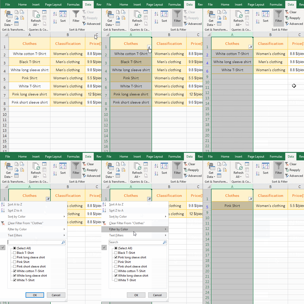
Figure 11

4. If you want to filter clothes ending with a certain word(such as "shirt"), the wildcard can be written as "*shirt". This filtering method can also be used to filter numbers.

(III) How to search multiple items in excel filter(Add current selection to filter)

This feature combines the results of several filters. If you want to filter the employees of the "Finance and Technology department". Select column B, select the "Data" tab, click the "Filter" icon, add this icon to column B, click the icon, enter "fi" in the input box of the expand menu, press enter "OK", click the Filter icon in column B again, enter "te*", check "Add current selection to filter", click "OK" to filter out all employees of "Finance and Technology department"; operation process steps, see screenshot in Figure 12:

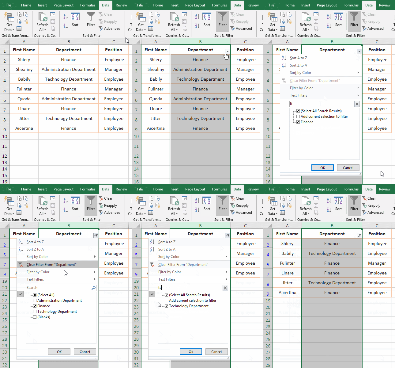
Figure 12

III, How to use Excel filter shortcut keys to operate

(I) Expand the "Filter" drop-down menu shortcut operation

1. If you want to filter employees whose "Total sales" is greater than 50000. Click the column number C of the third column, select the third column, and press the shortcut keys Ctrl + Shift + L, then add a filter icon to column C; press Alt + down arrow to expand the "Filter" drop-down menu, release the first two keys, press F, expand the submenu, press the first letter of each option, select the item, for example, press g to select "Greater Than", then press Enter, open the "Custom AutoFilter" dialog, enter 50000 on the right side of "is greater than", press Enter, it will automatically filter out all employees whose sales performance is above $50,000; the operation steps are as shown in Figure 13:

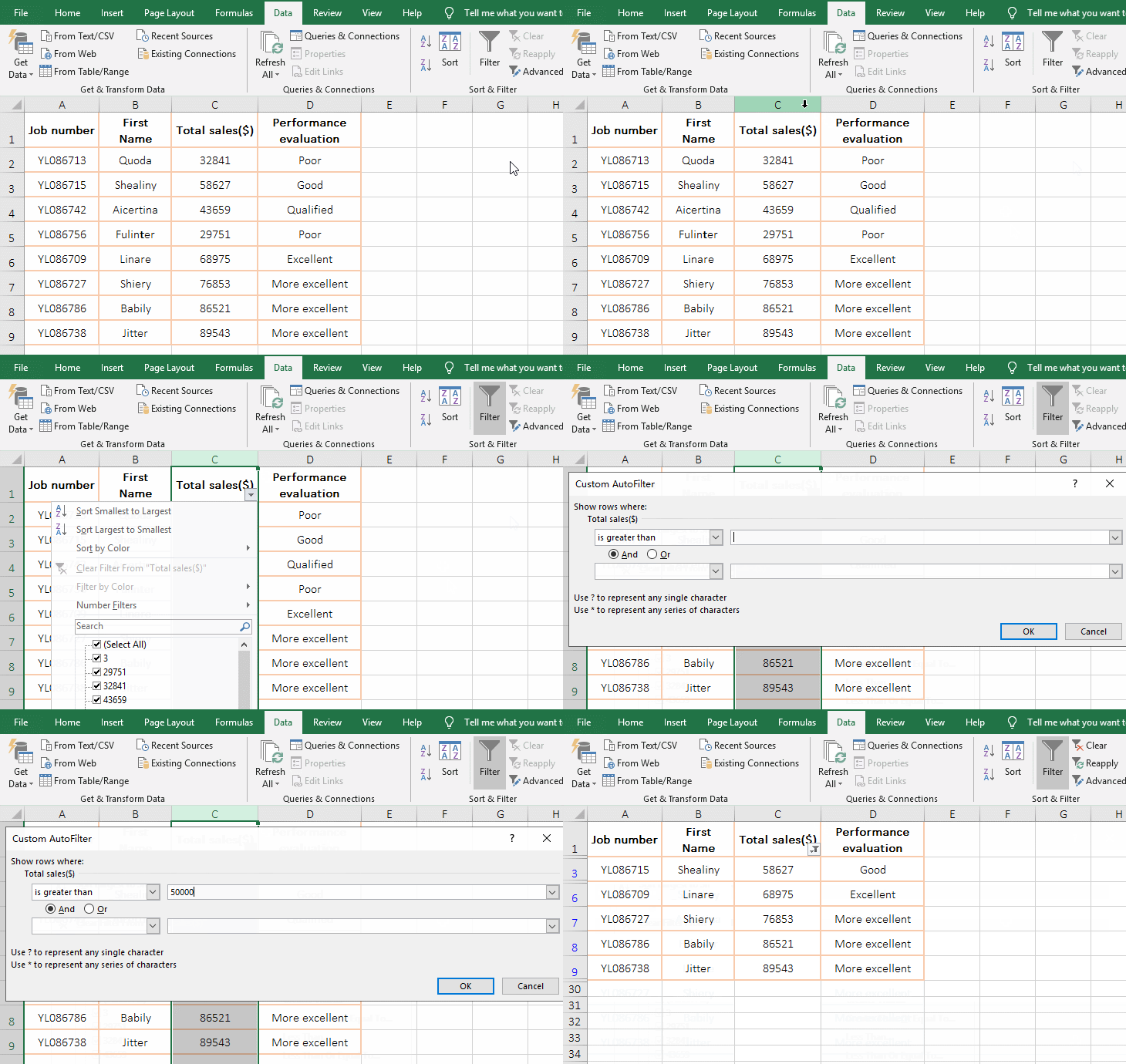
Figure 13

2. If the selected column is text, the same method is used. At this time, the F key indicates text filter. After expanding the Filter drop-down menu, if you filter by color, press I to expand the submenu and select the appropriate option.

(II) "Filter" in the right button menu of mouse is operated with shortcut keys

1. If you are asked to only select students with the English score of 659. Select one of the English scores(such as B2) with 659 points, press Shift + F10, expand the right button menu of mouse, release the first two keys, press E, expand the filter sub-option, press V to select "Filter by selected cells' Value", it will automatically filter out all students with the English score of 659; the process steps are shown in Figure 14:

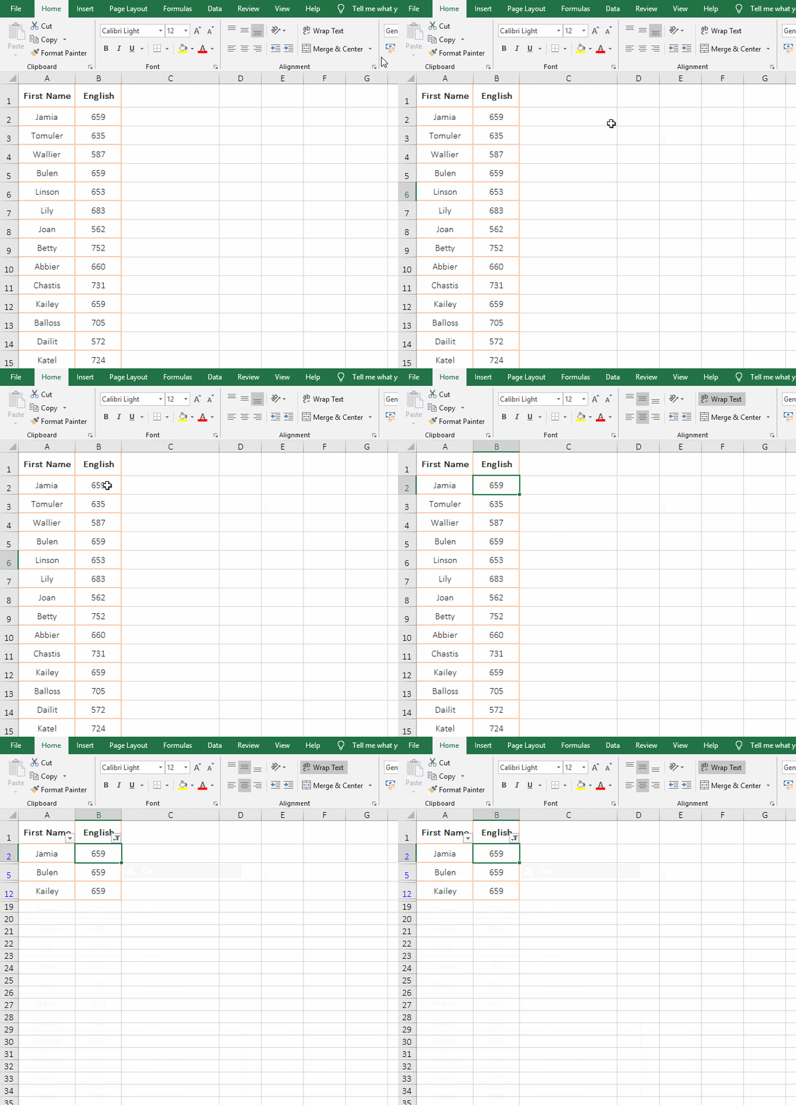
Figure 14

2. If you want to use the shortcut keys to operate other filtering options in the right button menu of mouse, expand the "Filter" submenu according to the method in the demo, and select the first letter of the last word of each option.

IV, Excel multi-column and multi-criteria filter

1. If you want to filter the students whose scores of "Advanced Mathematics and English" greater than or equal to 700. Select one of the cells in the table, press Ctrl + Shift + L to add a filter icon to each column of the table; click the Filter icon in column B, and select "Number Filters" → "Greater than or Equal To" in the expanded menu, open the "Custom AutoFilter"dialog, enter 700 on the right side of "is greater than or equal to", it will automatically filter out all students whose scores of "Advanced Mathematics" are greater than or equal to 700; click the "filter" icon in column C, filter the students with "English" greater than or equal to 700 points with the same method; this will filter out all students who meet the two criteria; the process steps, see screenshot in Figure 15:

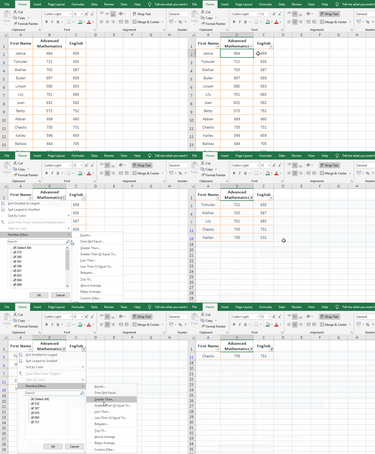
Figure 15

2. In addition, search filters can also filter data that meets multiple criteria simultaneously in multiple columns, just add a filter icon to each column.

V, How to delete filtered data in excel

1. Clear the filter. Click the Filter icon in column B, select "Clear Filter From "Advanced Mathematics" in the expanded menu, then the filter in column B is cleared; then click the "Filter" icon in column C, Select "Clear Filter From English" in the expanded menu and the filter in column C is cleared; the operation is shown in Figure 16:

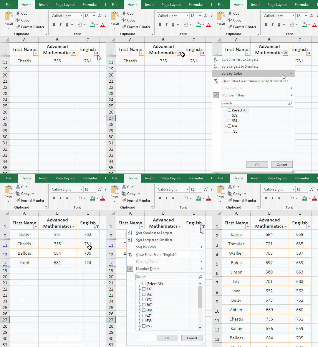
Figure 16

2. Delete the Filter icon. Select one of the cells in the table and press the shortcut keys Ctrl + Shift + L, the "filter" of each column of the table is deleted. The operation steps are as shown in Figure 17:

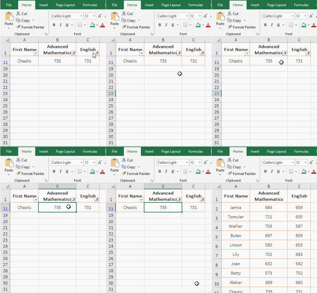
Figure 17

In addition, after selecting any cell of the table, select the "Data" tab, and click the "Filter" icon once to delete all the "Filter" of the table.