Combine multiple excel sheets into one pivot table with multiple consolidation ranges in excel

You can combine multiple excel sheets into one pivot table with multiple consolidation ranges in excel. There are two ways to merge, one for merging with a single page field and the other for merging with the page fields. Singlepage fieldis used to merge tables with only one level or one category, and the page fields are used to merge two-level to four-level or two to four categories.

After combining multiple tables into a pivot table, you can summarize them according to different requirements. For example, it can be summarized by region or city, summarized by year or quarter, summarized by category, summarized by one product, etc. The following are two examples of summarizing by month or by region or city in region.

I, Combine multiple excel sheets into one pivot table with in excel

(I) Create a pivot table of single page field(only one level or one type)

1. If you combine the sales of clothing from April to June into a pivot table. Switch to the first table "April" to be combined, hold down Alt, press D and P once, open the "PivotTable and PivotChart Wizard - Step 1 of 3" dialog, and select "Multiple consolidation ranges", select "PivotTable" for "What kind of report do you want to create";

2. Click "Next", go to "Step 2 of 3", select "Create a single page field for me" for "How many page fields do you want"; click "Next" to go to "Step 2b of 3" dialog. Select A1:B8, then "April!$A$1:$B$8" is automatically filled in the "Range" input box, click "Add" to add the "April!$A$1:$B$8" to "All ranges", then switch to the "May and June" worksheets in turn, and add the ranges to be combined to "All ranges" in the same way;

3. Click "Next", go to "Step 3 of 3" dialog, select "New Worksheet", click "Finish", then start to combine the selected table into PivotTable, after a while, the merger is completed. See screenshot in Figure 1:

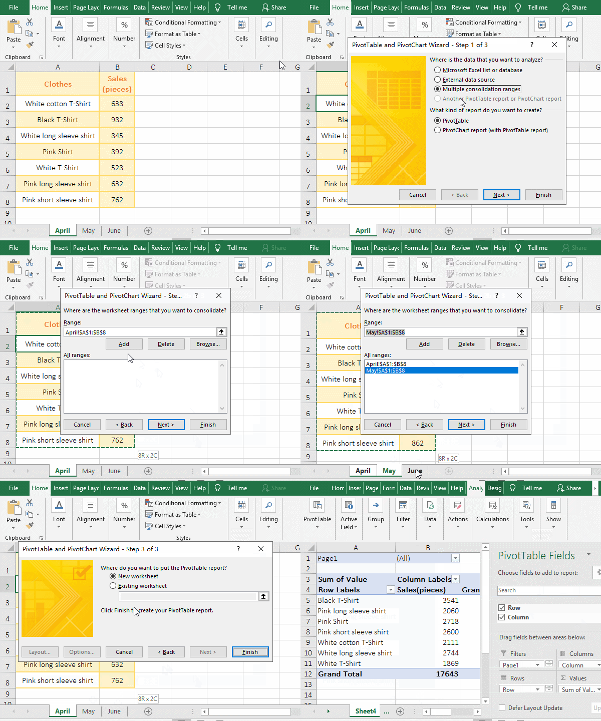
Figure 1

4. Description: "Create a single page field" has only one "page field"(ie "Page 1"), which is used when there is only one level or one category. For example, from April to June in the demo belongs to the second quarter, so combine them into "Page 1". If you want to summarize the sales for each quarter of the year, you will use "the Page Fields" to define two page fields, which are divided into two levels, please see below.

Hint: If the table to be combined is not open, select "Browse" to add a reference to the range of table after adding the excel document to the "Range", otherwise, the message "Consolidation reference is not valid" is displayed, see screenshot in Figure 2:

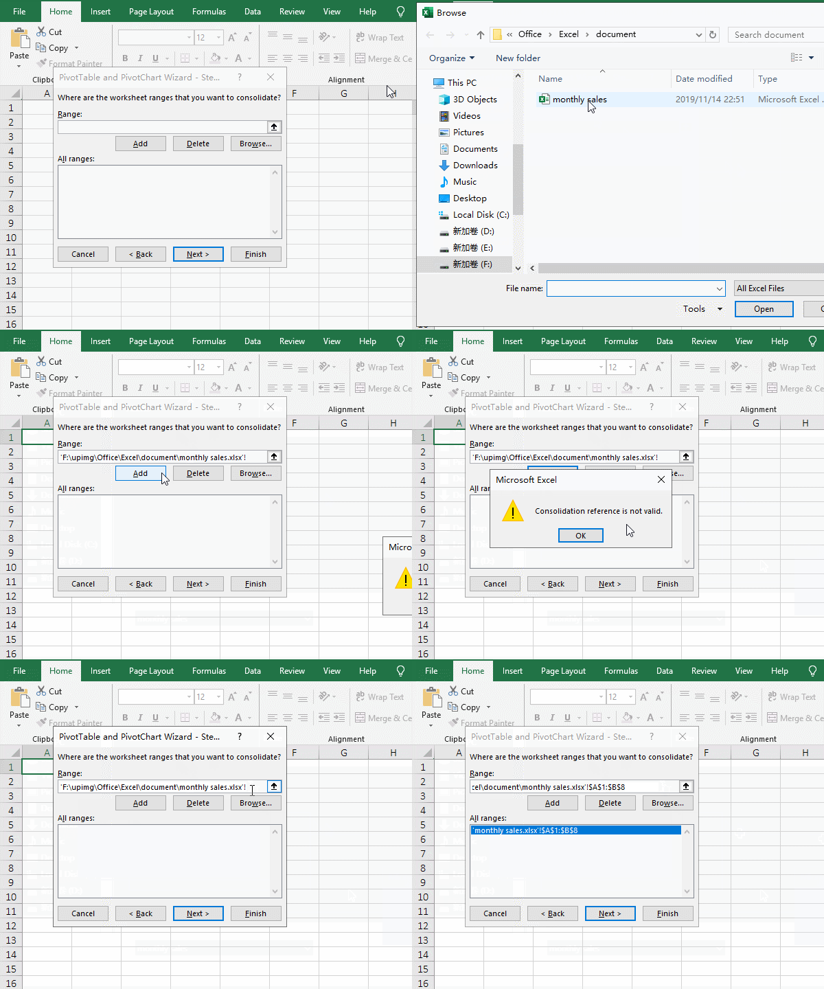
Figure 2

(II) Create one pivot table of the page fields(two levels[or two types] or more)

1. If you want to combine the sales and turnover of clothing in each region and city. Switch to the first table to be combined(such as "New York"), hold down Alt, press D and P respectively, open the "PivotTable and PivotChart Wizard" dialog, select "Multiple Consolidation ranges", click "Next";

2. Go to "PivotTable and PivotChart Wizard - Step 2a of 3", select "I will create the page fields"; click "Next", go to "Step 2b of 3"; select A2:C9, "Please specify the name to be built in the PivotTable. select 2 for "How many page fields" do you want", copy "Middle Atlantic" to "Field one", enter "New York" for "Field two", click "Add", the range to be selected and the content to be inputted are successfully added;

3. Click the worksheet label "Philadelphia" to switch to the worksheet, also select A2:C9, select "New York" in "Field Two", enter "Philadelphia", click "Add", and successfully add the data of "Philadelphia";

4. Add page 2. Click the worksheet "Los Angeles" to switch to this table, the worksheet name in the "Selected Range" will automatically change to "Los Angeles"(ie 'Los Angeles'!$A$2:$C$9), and the selected range is the same as "Philadelphia", so no need to select,  enter "Pacific" in "Field one", change the "field two" to "Los Angeles", click "Add", successfully add the data of "Los Angeles"; click the worksheet "Seattle" to switch to it, "Seattle" is automatically filled to the "Sselected Range", enter "Seattle" in "Field two", click "Add", then successfully add the data of "Seattle"; click the worksheet "San Francisco" to switch to it, "San Francisco" is automatically filled in the "Selected Range", enter "San Francisco" in "Field two", click "Add", then successfully add the data of "San Francisco";

5. Check whether the region corresponds to the city. In the "All Ranges" list box, the current option is "San Francisco!$A$2:$C$9", which already corresponds to the two options "Field one" and "Field two"; select "Seattle!$A$2:$C$9", its "Field one" is "Pacific", but "Field two" is "San Francisco". Click the drop-down list box of "Field tow" and select "Seattle"; the rest is also checked.

6. Create a pivot table. Click "Next", select "New Worksheet" for "Where do you want to put the PivotTable report", click "Finish", then combine all selected tables into one PivotTable; the operation steps are as shown in Figure 3:

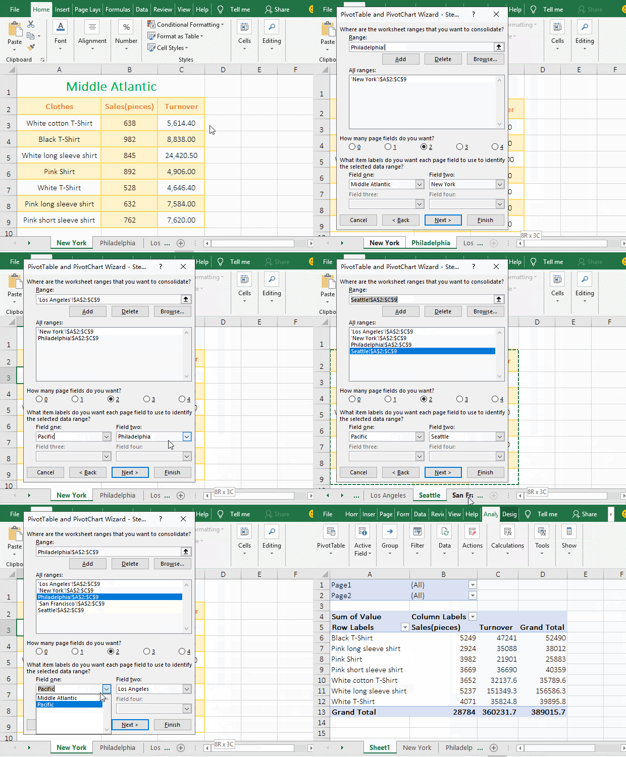
Figure 3

7. Description: "The page fields" is used to combine multiple tables that are levelled or classified two or more. It can set up 4 fields, each field represents one level or one class, so you can combine the multiple tables that are levelled or classified into four into one pivot table. For example, the table in the demo is divided into two levels(ie, region and city), if you want to add a larger region or year, you can select 3 fields.

Tip: If you want to modify the combined PivotTable, hold down Alt, press D and P respectively again, open the "PivotTable and PivotChart Wizard" dialog again, and click "Back" to switch to the dialog to be modified, just fine.

II, Excel adjusts the PivotTable and subtotal it as required

(I) Adjust the pivot table of the single page field and subtotal

1. Adjust the field to display the page, row and column to a table

A. move the mouse to the "Column" in the area "Columns", hold down the left button, and then drag to the area "Rows", when a bold green line appears, then release the left button, the same method put "Page1" drag from the "Filters" to the area "Columns";

B. Right-click one of the cells(such as A3), select "Pivot Table Options" from the pop-up menu, select the "Display" tab in the dialog that opens, and check "Classic PivotTable Layout(enables dragging of the fields in the grid)", click "OK"; right click on any cell in the table, select "Subtotal "Row"" in the pop-up menu, then cancel the "Row" subtotal, the page, row and column are displayed to a table; Operation process steps, see screenshot in Figure 4:

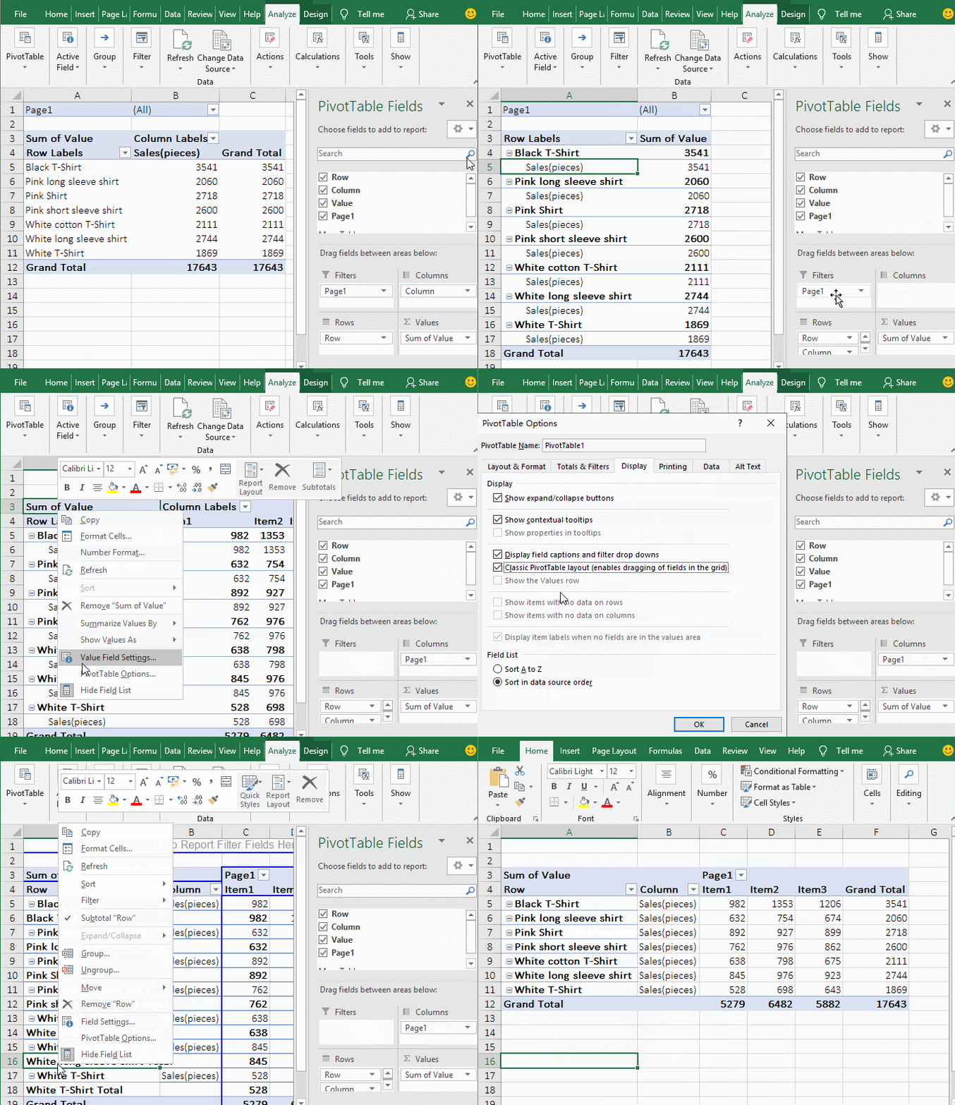
Figure 4

2. Modify the name

Select A4, select the "Analyze" tab, change "Row" to "Clothes" under "Active Fields" in the top left of the screen, select B4, change "Column" to "Unit", and then select C3, then change "Page1" to "Month"; select C4, enter "April", change "item 1" to "April"(if you cann't input, you can hold down Ctrl, click C4, then input), and change "item 2 and item 3" to  "May and June" in the same way respectively; the operation process steps, see screenshot in Figure 5:

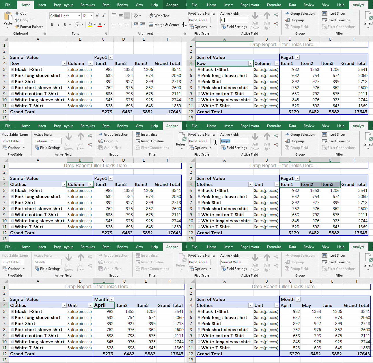
Figure 5

3. Adjust the line height and alignment

Click row number 3 to select the third row, hold down Shift, then click row number 12, select the table, right click on one of the row numbers, select "Row Height" in the pop-up menu, enter 24, press Enter, the rows height are adjusted to 24; select the "Home" tab, click the "Middle Align and Center" icons, and center each column horizontally and vertically; the operation steps are as shown in Figure 6:

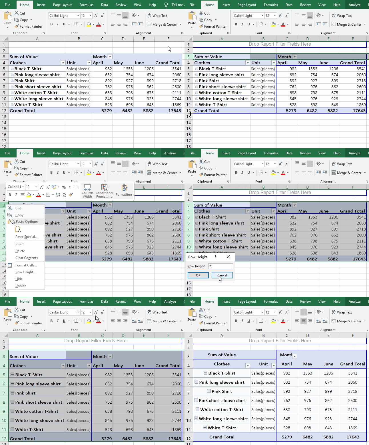
Figure 6

(II) Adjust the PivotTable of the page fields and subtotal

1. Modify the name

Select cell A1, enter "Region", press Enter, enter "City"; select A5, enter "Clothes", press Enter, modify the name to complete; the operation process steps, see screenshot in Figure 7:

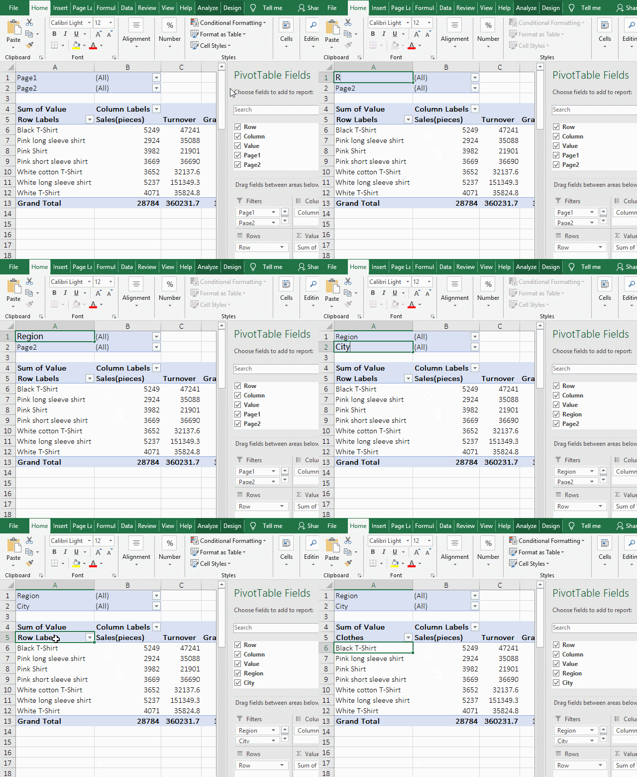
Figure 7

Tip: If the version of excel is 2016 and before 2016, the method of operation is: Double-click the blank space of the A1 cell(do not double-click the text), position the cursor behind the text, select "Page1", and enter "Region"; in the same way, change "Page2" to "City"; double-click A5, select "Row Label", change it to "Clothes", press Enter, modify the name to complete.

2. Adjust the position of the field according to different subtotal requirements

A. Subtotal sales and turnover in each city

(1) Drag the "City" field from the "Rows" to the "Columns" and place it on top of the "Column"; right click D5, select "Subtotal "City"" in the pop-up menu, the meaningless subtotals city are canceled because they accumulate sales volume and turnover; right click L5, select "Remove Grand Total" in the pop-up menu, and delete the meaningless "column total"; the operation steps are as shown in Figure 8:

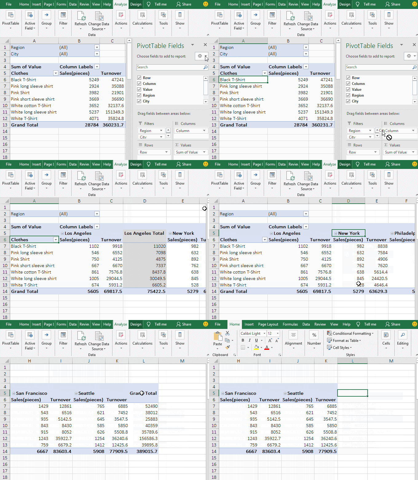
Figure 8

(2) Adjust the column position. If you want to transfer "Los Angeles" to the right of "Philadelphia"; click B5 to select it, while holding down the left button, select B5:C14, move the mouse to the right line of the selected range, hold down Shift and left button of mouse, drag right until drag to the right line of column G, when the long bold green line appears, then release the left button, the position adjustment is successful; the operation process steps, see screenshot in Figure 9:

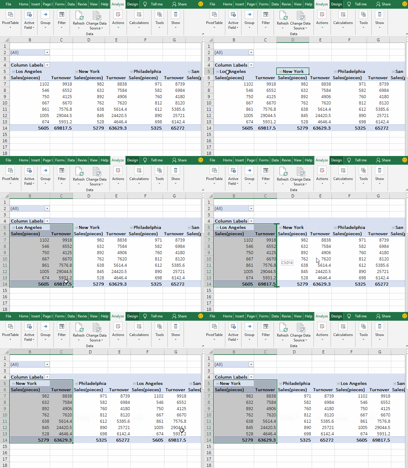
Figure 9

(3) Filter demonstration. Click the filter icon in B2, select "Middle Atlantic" from the pop-up menu, and click "OK" to filter out the records of "Middle Atlantic"; the same method select "Pacific" to filter out the records of "Pacific"; operation process steps, as shown in Figure 10:

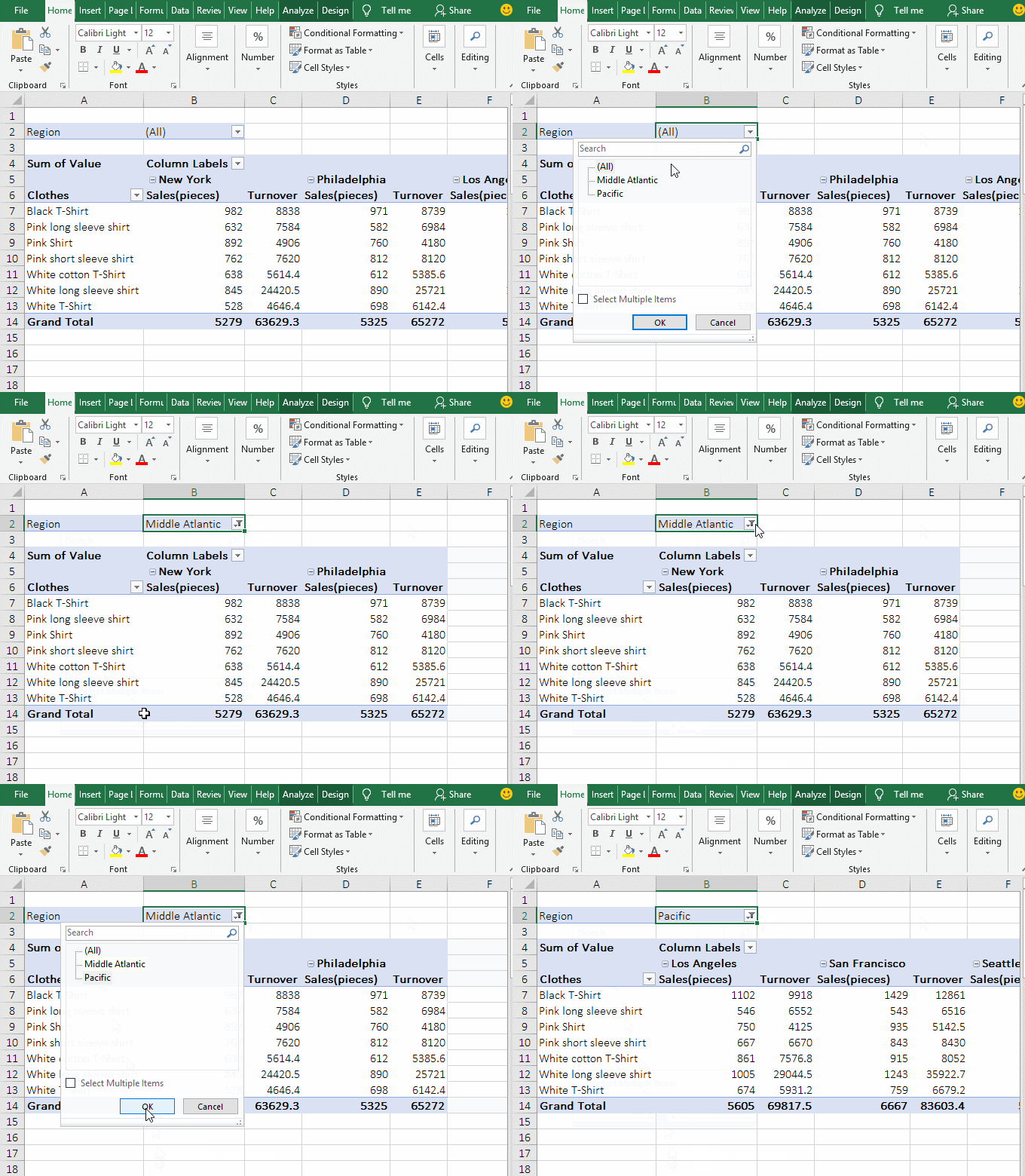
Figure 10

B. Subtotal sales and turnover of each garment in all cities

Drag the "City" field from "Column Interval" to "Line Interval" to summarize the sales and turnover of each garment in all cities; the operational steps are shown in Figure 11:

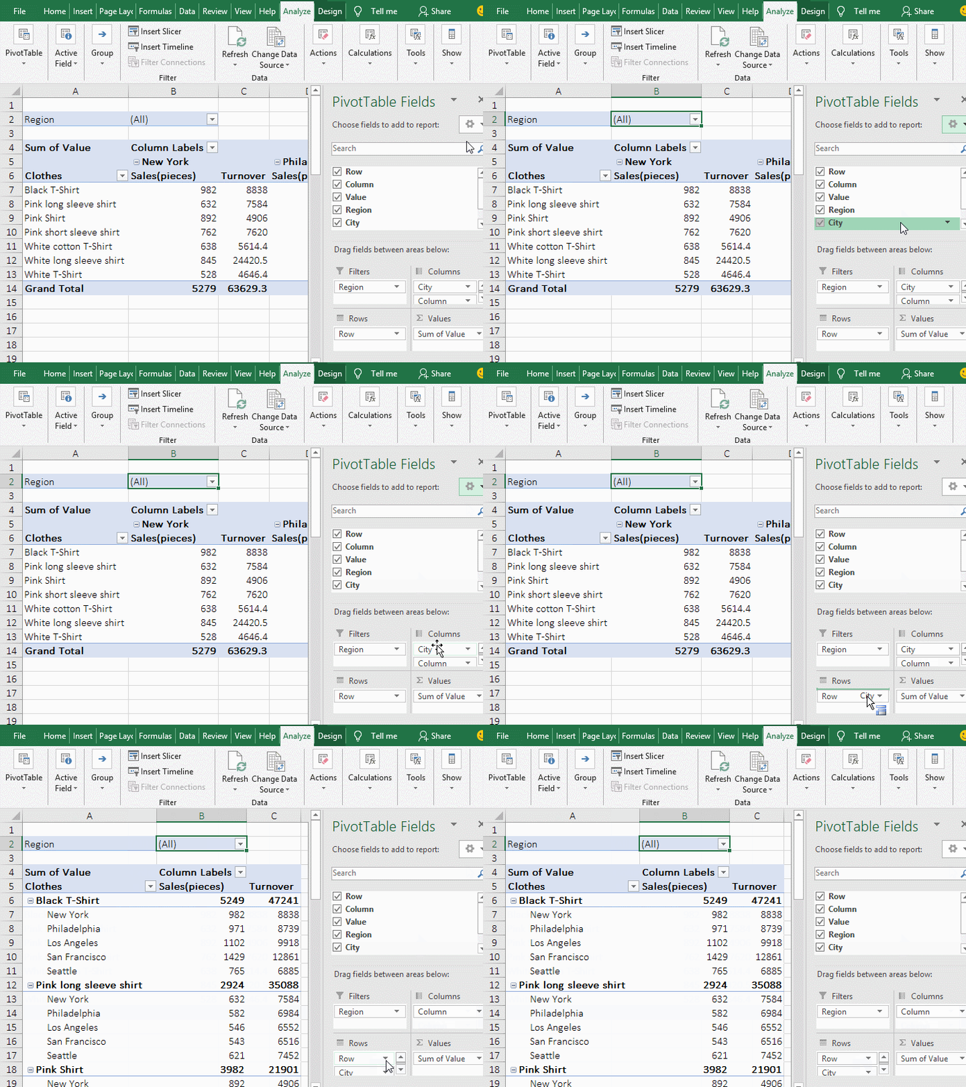
Figure 11