 Office > Excel > Excel 2019 > Content
How to create a pivot table in excel(15 examples, with distinct count, percentage and four areas)
Pivot Table are used to make statistics in excel, such as counting the percentage of employees in each department as a percentage of total employees, the percentage of sales per product to total sales, and sales in a certain area of each product accounted for percentage of sales in all areas, etc. Its computational classes have sum, average, count, max, min, product, stddev, and distinct count.
How to do a pivot table in excel? It can be created in two ways, one is to create an empty pivot table, and the other is to create a pivot table recommended by excel, which is a pivot table that is statistically calculated according to certain items. If you create an empty PivotTable, you need to count the items you want to count. To complete the statistics, you need to know the usage between the four areas, the choice of calculation type, and the choice of how to show the values etc. The article lists the two examples that are the statistics of distinct count and percentage.
I, How to create a pivot table in excel
(I) Create an empty pivot table
(1) Create a Pivot Table to another worksheet
1. Select one of the cells of the table you want to create the Pivot Table(such as A2), select the "Insert" tab, click "PivotTable" in the upper left corner of the screen, open the "Create PivotTable"dialog, "Table/Range" has automatically filled out the reference to the table(ie Sales!$A$1:$E$10); select "New Worksheet" for "Choose where you want the PivotTable report to be placed" and check "Add this data to the Data Model", click "OK" to start creating the PivotTable. The length of time depends on the size of the table. After the PivotTable is created, it will automatically switch to the worksheet. By default, no fields are selected, check the "Classification and Sales", then count the "Sales" of each clothes; the operation process steps, see screenshot in Figure 1:
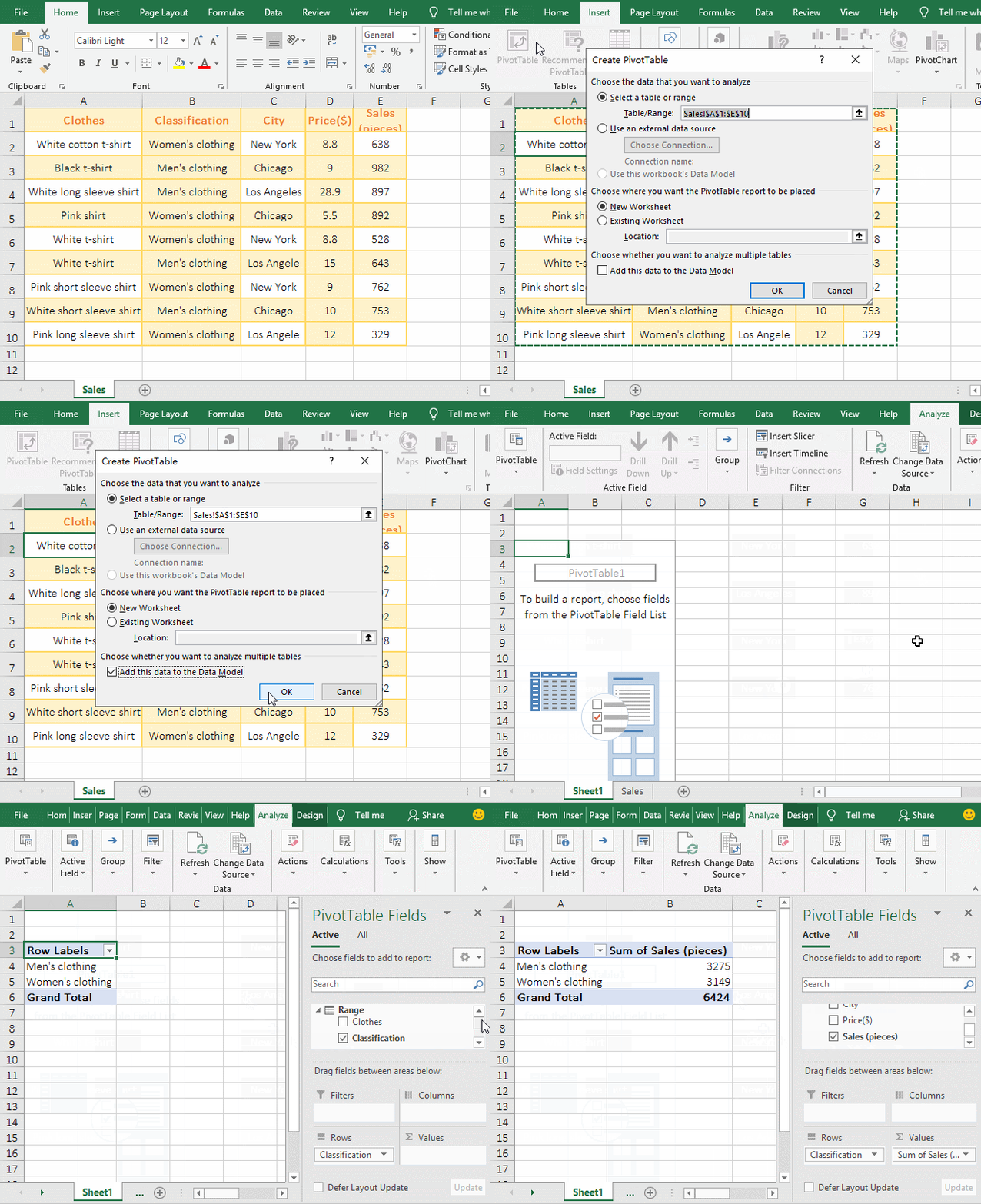
Figure 1
2. Description:
A. If you don't create a PivotTable for the entire table, just create some cells or columns, you can just select them; for example, only create the PivotTable for columns A, B, and C, just select these three columns.
B. If you check "Use an external data source", you can use another excel document or database as the data source for creating a PivotTable. If you want to use the database as a data source, you need to establish a connection to the database.
C. The function of "Add this data to the Data Model" is Distinct Count, that is, duplicate items are counted only once. If the table has duplicate data, you can check it; if not checked, there will be no "Distinct Count" in the value list.
Tip: To open the "Create PivotTable" dialog, you can also press the shortcut keys Alt + N + V. The keystroke method is: hold down Alt and press N and V one time.
(2) Create a PivotTable to an existing worksheet
1. If you only create a pivot table for columns C, D, and E. Click column number C, select column C, hold down Shift, click column number E, select columns C, D, and E. Hold down Alt and press N and V respectively to open the "Create PivotTable" dialog. Select "Existing Worksheet", click the input box to the right of "Location" to position the cursor there, click G1, then Sheet1!$G$1 is automatically filled in, indicating that the PivotTable is created to G1, click "OK", successfully create the PivotTable, check "City and Sales", counts the sales of each city; steps, see screenshot in Figure 2:
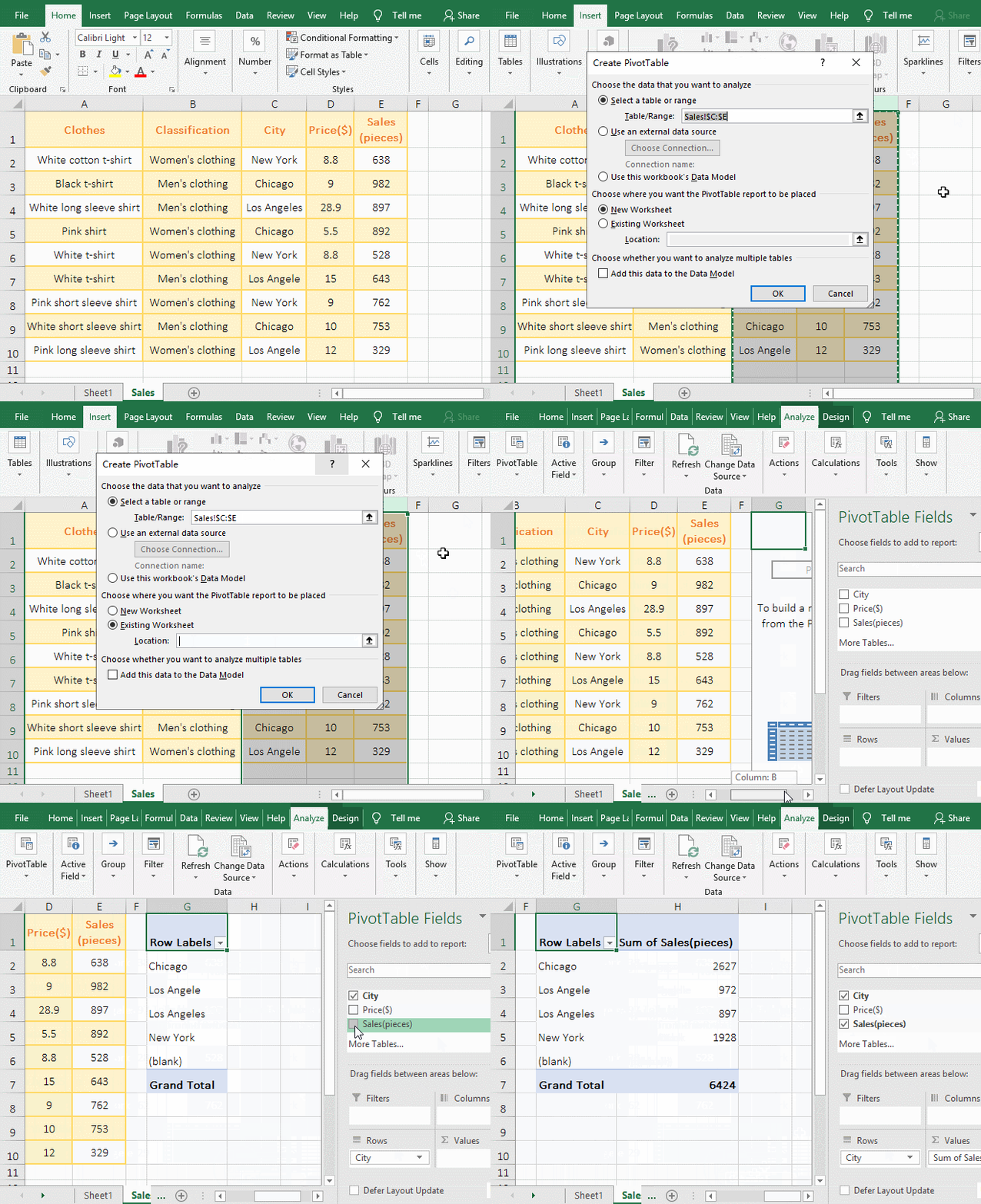
Figure 2
2. If you only create a PivotTable with a few columns, these columns must be continuous, otherwise you can't create them. Discontinuous columns, you can move together. Hold Shift and move the mouse to the left or right line of the column you want to move, after the mouse becomes a small plus icon, press and hold the left button to move.
(II) Create a "Recommended PivotTable"
1. Select one of the cells you want to create the PivotTable, select the "Insert" tab, click the "Recommended PivotTables" in the upper left corner of the screen, open the "Recommended PivotTables" dialog, and select a Pivot Table style(such as "Sum of Sales(pieces) by City"), click "OK", then create a PivotTable of the selected style, it has already counted the "Sales" for each city ; operation process steps, see screenshot in Figure 3:
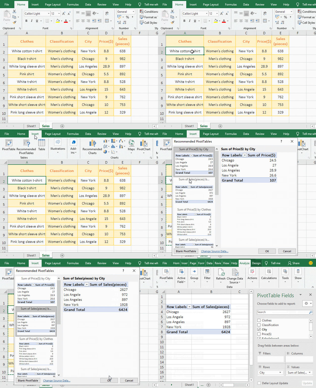
Figure 3
2. Description: The "Recommended PivotTable" is actually a table with one or more items that are well counted. For example, the "Sum of Sales(pieces) by City" in the demo is that the sales of each city have counted. If the "Recommended PivotTable" has an existing style, choosing a PivotTable to create is faster.
Tip: To create a "Recommended PivotTable" you can also use the shortcut keys Alt + N + SP, the keystroke method is: hold down Alt and press N, S and P one time.
II, How to change the data source and update after source table to be modified after you create a pivot table in excel
(1) How to change excel pivot table data source
Suppose you want to change the data source from the entire table to column A to D. Click one of the cells in the PivotTable (such as A3) to display the "Analyze" tab, select ""Analyze", click the "Change Data Source" icon, and Excel automatically switches to the data source table, select column A to D, click "OK", then the data source is changed to column A to column D. The "Sales" column is gone; the operation steps are as shown in Figure 4:
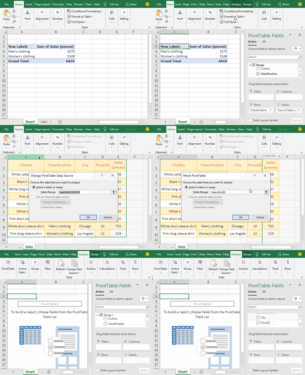
Figure 4
(2) How to update pivot table in excel after source table to be modified
1. Take the example of deleting the record "White long sleeve shirt" that belongs to "Men's clothing" in the source table as an example. Right-click row number 2, select "Delete" in the pop-up menu, delete the record; click the "PivotTable" tab to switch to the worksheet, select the "Men's clothing" corresponding to cell B4, select the "Analysis" tab, click "Refresh", then the "Sales of Men's clothing" reduce, indicating that the PivotTable has been updated; the operation process steps, as shown in Figure 5:
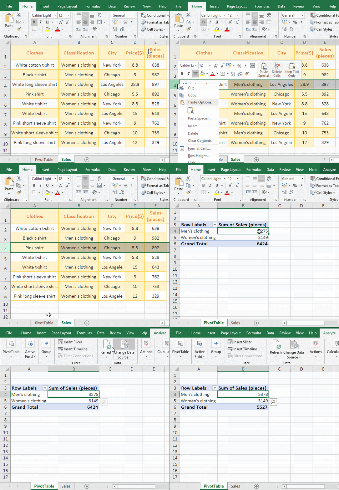
Figure 5
Tip: If you add a record after the table, you need to update the data source because the added record is not in the range of the selected table.
2. If you want to automatically refresh the data when opening the document, you need to set, the method is that right-click the cell A3(ie "Row Labels), and select "PivotTable Options" from the pop-up menu to open the "PivotTable Options" dialog, select the "Data" tab, check "Refresh data when opening the file", click "OK", the data will be automatically refreshed each time you open the document; the operation steps, see screenshot in Figure 6:
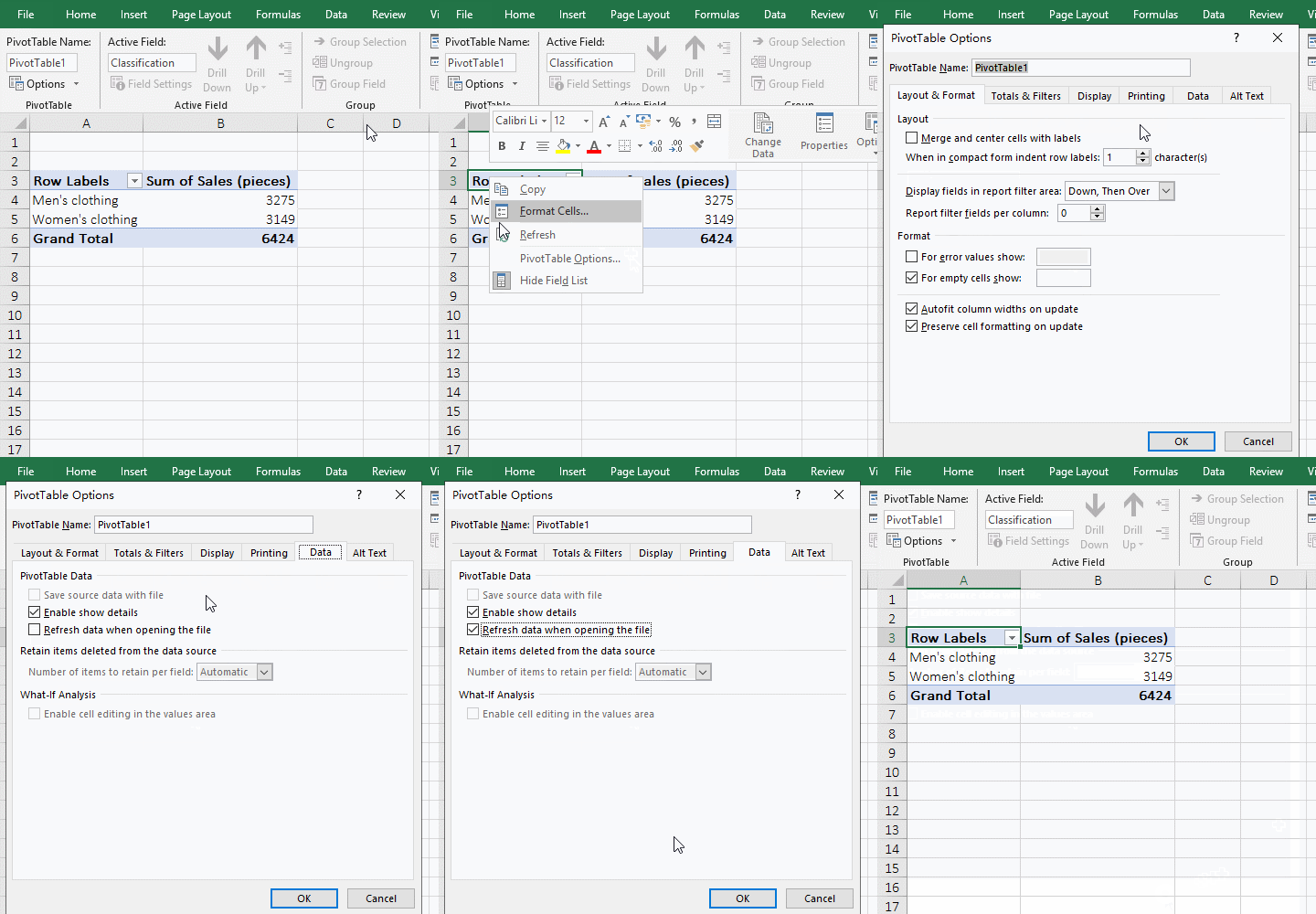
Figure 6
Tip: You can also use the shortcut keys Shift + F10 + O to open the "PivotTable Options" dialog, the method: press the Shift key and press F10 and O one time.
III, The four areas of Excel PivotTable
(1) The area "Rows"
The area "Rows" is used to display the field to the row. If it is a "text" field, it will be automatically displayed the row as long as it is checked; if it is a numeric field, it needs to be dragged to the area "Rows", it is only displayed the row. For example, check "Clothes", it will be automatically displayed to the area "Rows", and displayed the row in the table; in the area "Rows", the "Classification" is displayed above the "Clothes", and the same order is displayed in the table, drag the "Clothes" onto the "Classification" and the order in the table is also exchanged; the demo is shown in Figure 7:
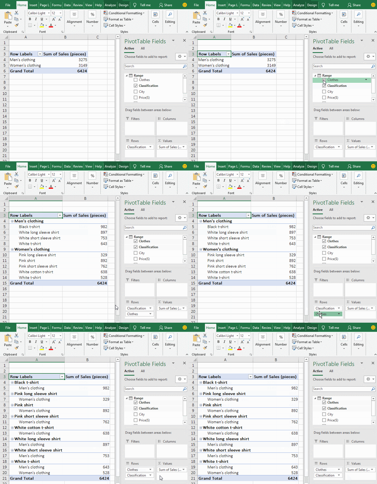
Figure 7
(2) The area "Columns"
The area "Columns" is used to display the fields to the column, just drag the field to be displayed to the column to the area "Columns", and each item of the field is displayed in a column. For example, drag "Clothes" to the area "Columns", each clothes's name is displayed in a column; the operation process steps are as shown in Figure 8:
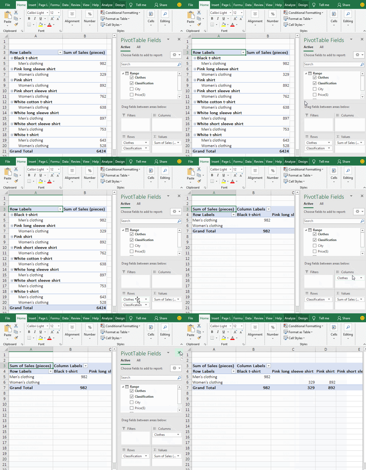
Figure 8
(3) The area "Filters"(Excel pivot table Filter)
1. The filter is used to filter the records, just drag the field to the area "Filters" to filter the records with this field. For example, drag "Classification" to "Filter", it will automatically display the "Classification" in A1, it will automatically display "All" in B1, click All, select "Select multiple Items", click the plus sign(+) in the pop-up menu to expand, click the checkbox in front of "All" to deselect all, and then check the "Men's clothing" to filter out all sales of the "Men's clothing"; the process steps are as shown in Figure 9:
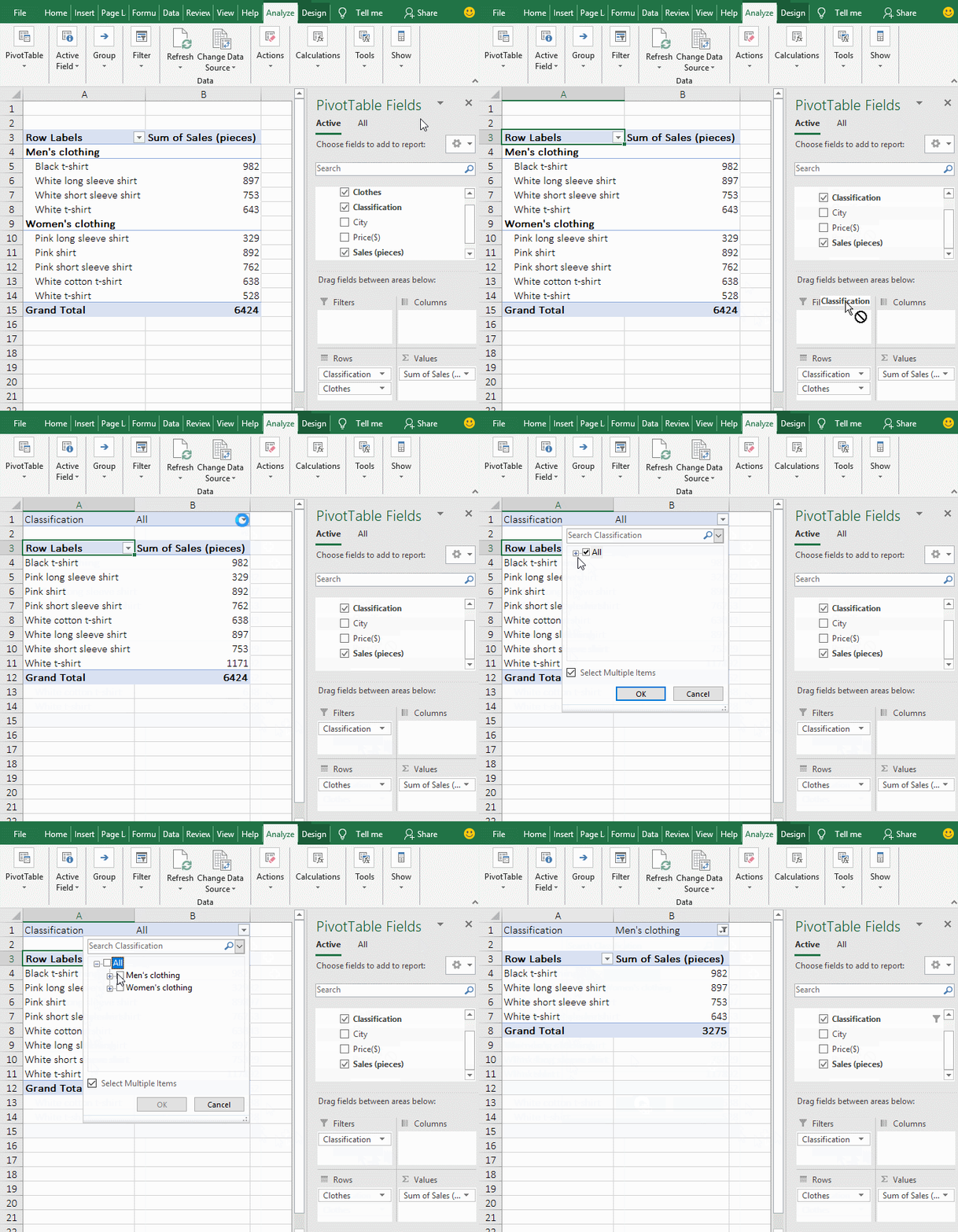
Figure 9
Tip: If you remove a field(such as "Classification") from the "Filters", you can filter from the "Row Labels" in A3 or re-pop the field to the "Filters".
2. "Quick Explore" can also add fields to the "Filters". Right-click the cell you want to quickly explore, such as A4(or click the magnifying glass icon on the right side of A5), expand the "Explore" dialog, select "Clothes", and then click "Drill to", then the "Men's clothing" in A4 is Selected as a filter, the "Classification" field is also added to the "Filters"; the process steps, see screenshot in Figure 10:
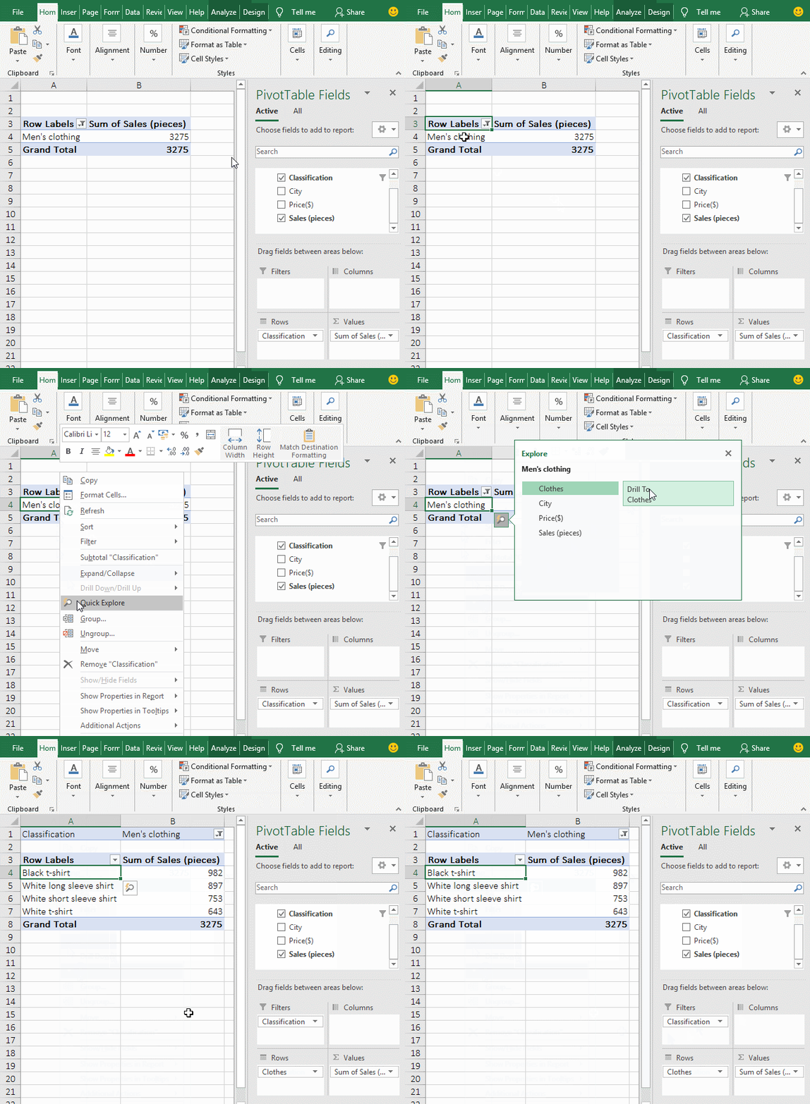
Figure 10
Tip: Fields that are not checked can be drilled.
Recovery after "Quick Explore". Drag the "Classification" from "Filters" to "Rows", click the filter icon in A3, and click "Select All" in the pop-up menu to check all Classification, then show all Classification and clothes belonging to them; Operation process steps, as shown in Figure 11:
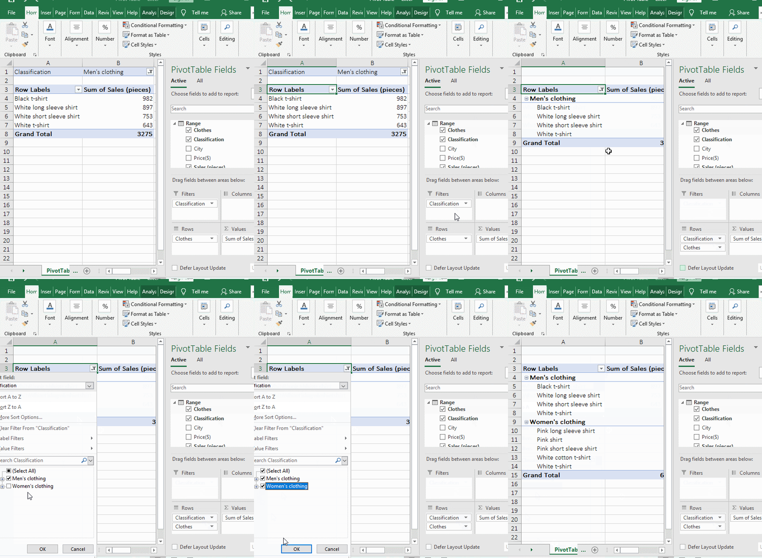
Figure 11
3. Double-click the "Value" column to display a complete record. If you want to fully display the information of each field of the clothing "Black t-shirt"; double-click the "sales in B5" corresponding to "Black t-shirt", excel will start to create a new worksheet(ie Sheet1), which shows all the information of "Black t-shirt"; the operation steps are as shown in Figure 12:
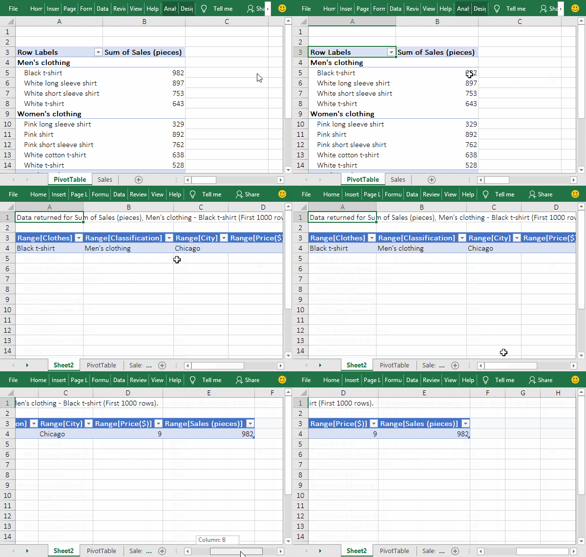
IV, Excel Pivot Table count
(1) Sum and average
1. If you want to change the sum to average. Double-click the title which you want change the calculation type(such as cell B3), open the "Value Field Settings" dialog, select "Average" under "Calculation Type", click "OK" to count the average sales of each city; the operation process steps are as shown in Figure 13:
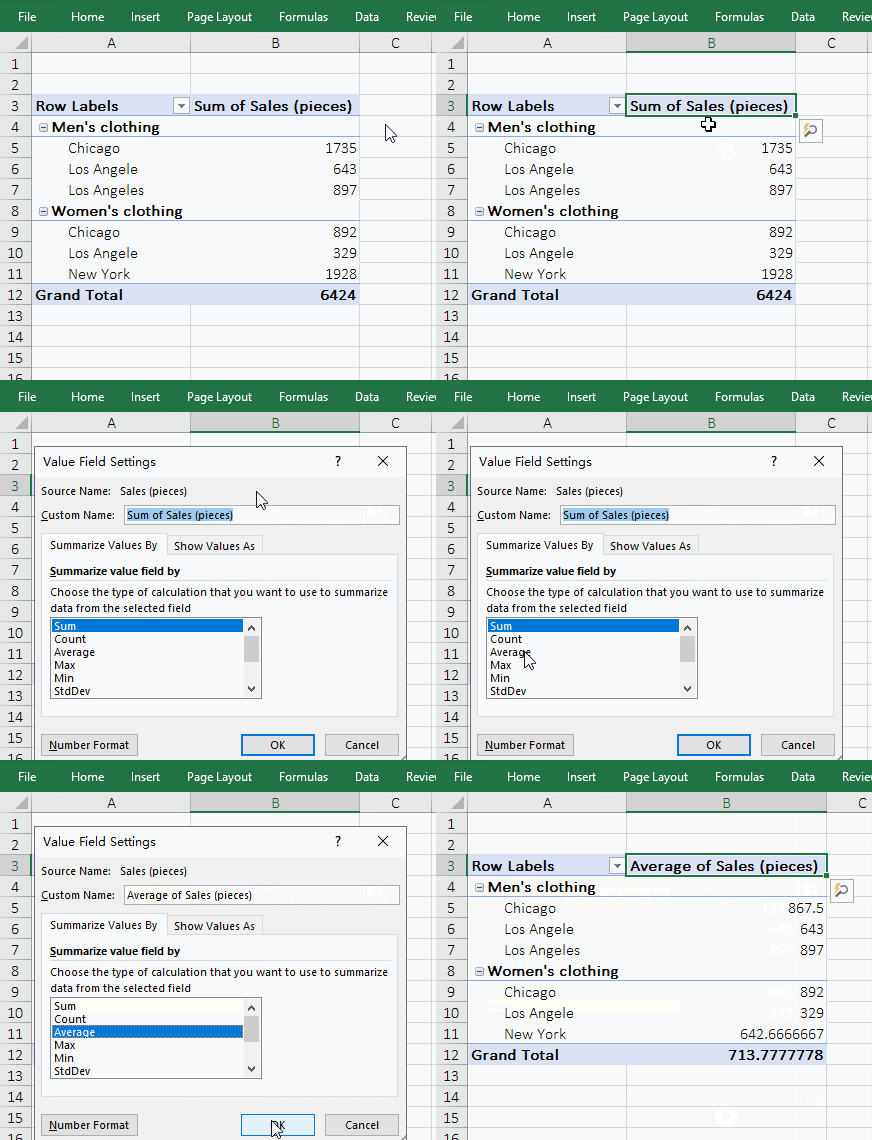
Figure 13
2. In the "Value Field Settings" dialog, there are a variety of "calculation types", you need to modify the type, you can choose.
(2) Excel pivot table count unique
If you want to distinct count the "Clothes". Drag the "Clothes" field to the "Σ Value" list and automatically count the number of each clothes, because "Count" is selected for "Calculation Type" by default, the clothes "Black t-shirt" has a statistical result of 2; double-click the cell B3 where the title of "Count" is located, open the "Value Field Settings" dialog, select "Distinct Count" for "Calculation Type", click "OK", then the repeated items will only be counted once, and the results of the clothes "Black t-shirt" is changed from 2 to 1; the operation process steps, see screentshot in Figure 14:
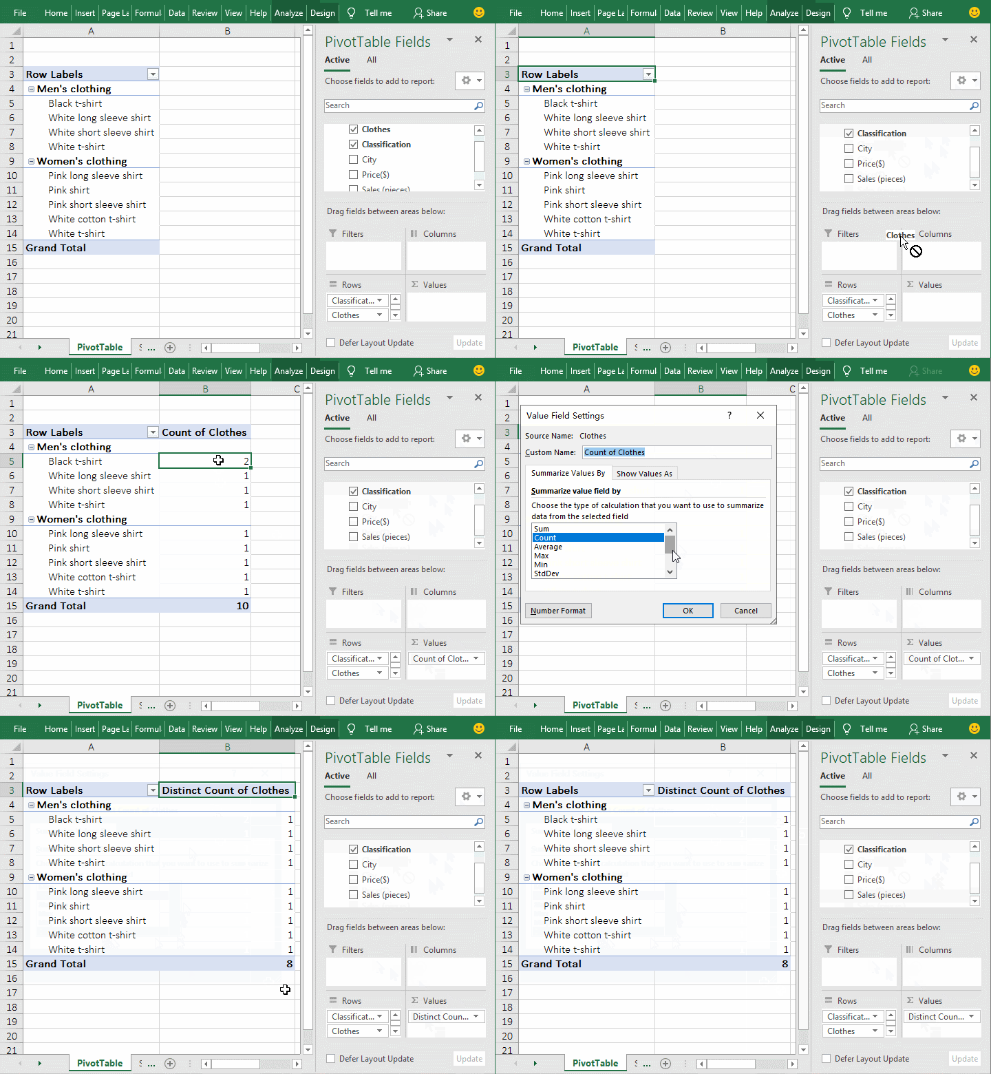
Figure 14
(3) Calculate percentage in excel pivot table
If you want to count the sales of each city's clothing as a percentage of total sales. Drag the "Sales(pieces)" field to the "Σ Value" list, double-click the cell C3 whose title is located, open the "Value Field Settings" dialog, change the "Custom Name" to "Percentage", click "OK", right click one of the cells of the value, such as C4, selects the "Show Values As → % of Grand Total" in the pop-up menu, then the percentage that meets the condition is counted; the operation process steps are as shown in Figure 15:
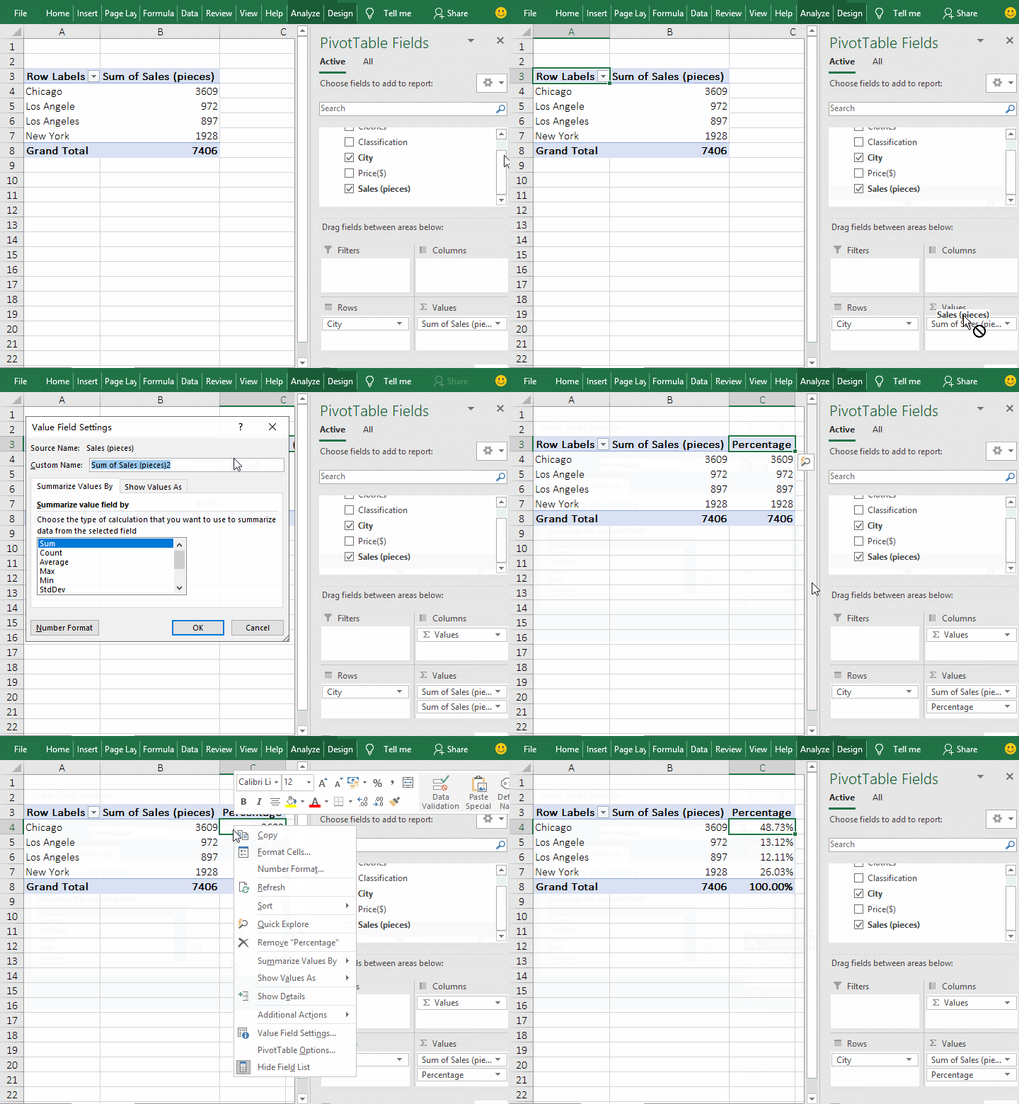
Figure 15
-
Related Reading
- Excel CountA and CountBlank function usage examples(
- 8 examples of Excel Match function, include it and S
- How to use offset function in excel, include it and
- Excel SumProduct function(multiple criteria, with if
- Excel left function usage(8 examples, with Sum+Value
- How to use Average function in excel(combine with if
- How to use advanced filter in excel(7 examples, mult
- How to use Excel address function(7 examples, with I
- How to filter in excel(16 examples, with number,text
- Excel SumIf function with ?/*, Average and array mul
- How to use Excel subtotal function(combine it with O
- How to use excel aggregate function(ignore error val