 Office > Excel > Excel 2019 > Content
How to use advanced filter in excel(7 examples, multiple criteria,copy to another worksheet,formula)
There are filter and advanced filter in excel, the difference between the two is that the filter can only be performed in the table range and only two criteria can be set; advanced filter can filter in the table range and copy the filtering results to another range or to another worksheet, and it can combine three or more criteria and also remove duplicates.
Excel Advanced Filter can either write criteria directly to cells or combine criteria with formulas. Its criteria can be text(such as a character or phrase), expression(such as not equal to null can be expressed as <>, equal to null can be expressed as =), formula(such as using And function or asterisk combination criteria formula). In the criteria, you can use the wildcard question mark(?) or asterisk(*); the question mark indicates any character, and the asterisk indicates any one or more characters.
I, How to use advanced filter in excel, display filtering results in the original range
(I) A criteria filter
1. Preparation criteria. There is an employee table, if you want to filter all employees of the "Finance Department"; select E1 cell, enter "Department", double-click E2, input or copy "Finance" to E2, then the criteria are ready.
2. Advanced filter settings. Click column number B of the second column, select the second column, select the "Data" tab, click "Advanced" in "Sort & Filter", open the "Advanced Filter" dialog, keep the default option "Filter the list, in-place" for "Action", and just selected cells(ie $B$1:$B$9) in the column B are automatically filled into the "List range", click the textbox on the right of "Criteria range", select E1:E2, then $E$1:$E$2 is automatically filled into the textbox, click "OK" or press Enter to filter out all employees of the "Finance"; the process steps are as shown in Figure 1:
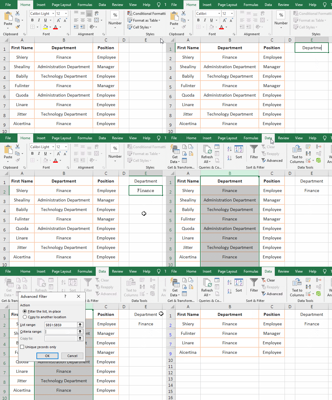
Figure 1
Hint: The field name of the criteria must be exactly the same as the field name of the filter column(the field name in the filter column has a line break character, and the field name of the criteria is also required). Otherwise, it will promot that the field name in the extraction range is missing or invalid and cannot be filtered. For example, the "Department" of the criteria is exactly the same as the field name "Department" of column B.
(II) Two criteria filter(Shortcut key for advanced filter in excel)
1. Preparation criteria. There is a student transcript, if you want to filter all students whose scores are above 680 in both "Advanced Mathematics" and "English". Enter "Advanced Mathematics and English" in E1 and F1 respectively, then copy >=680 to E2 and F2, and the criteria are ready.
2. Advanced filtering settings. Click the column B and hold down the left button, drag it to the column C, select the B and C columns, hold down the Alt key, press A and Q once, open the "Advanced Filter" dialog, click the textbox to the right of the "Criteria range" to position the cursor inside, select E1:F2, and the other keep the default values, and press enter to filter out all the students who meet the two criteria. The operation steps are as shown in Figure 2:
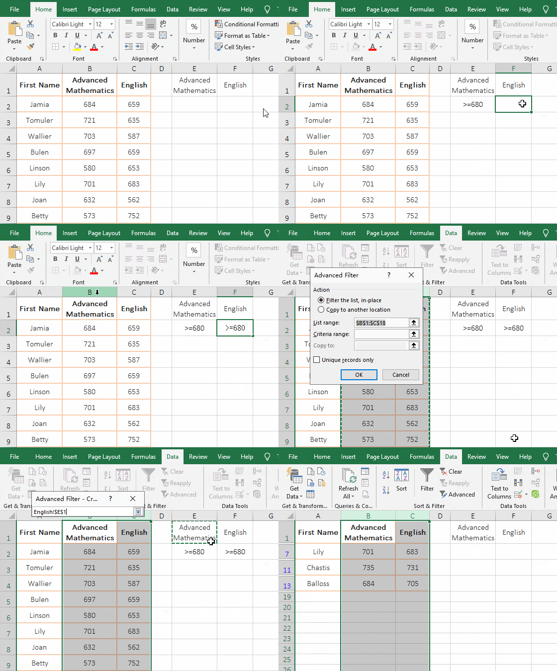
Figure 2
3. If you want to filter to meet three or more criteria, prepare these criteria and then select them to the criteria range.
II, Copy the filtering results to other locations, how to use advanced filter in excel
(I) Copy the filtering results to the same worksheet
1. Preparation conditions. Suppose you want to filter all clothes whose Classification are "Women's clothing" and "Price" are greater than and equal to 10. Enter "Classification and Price($)" for F1 and G1, enter "Women's clothing"(or ="=Women's clothing") in F2, and copy >=10 to G2, then the criteria are ready.
2. Advanced filtering settings. Click on the first column to select it, while holding down the left button, drag it to the last column of the table to select the table, hold down Alt, press A once, press Q once, open the "Advanced Filter" dialog, the "List range" has been automatically filled by the selected table range, click "Copy to another location" to select it, click the textbox on the right side of "Criteria range" to position the cursor here, select the criteria range F1:G2, then $F$1:$G $2 is automatically filled in the textbox, positions the cursor to the textbox to the right of "Copy to", clicks the cell I1, then $I$1 automatically is filled in the textbox, and selects "Unique records olny" to exclude duplicate data, click "OK", then filter out one garment that meet the criteria; the process steps, see screenshot in Figure 3:
Figure 3
Hint: The field name "Price($)", if there is a newline between "Price" and "($)", the criteria name(such as in K1) also has a newline, otherwise it will prompt the error that the field name in extract range is missing or invalid.
(II) Copy the filtering results to another worksheet(Advanced filter excel multiple criteria)
1. Preparation criteria. If you want to filter the clothes whose name start with "White", "Price" less than $10 and "Sales" greater than or equal to 600 to another table. Enter "name of clothes, price($) and sales(pieces)" for F1, G1 and H1 respectively, enter "white*" in F2 and <10 in G2, copy >=600 to H2, and the criteria are ready. * in "white*" is a wildcard character, indicating any one or more characters, "white*" means beginning with "white", and there can be any one or more characters after "white".
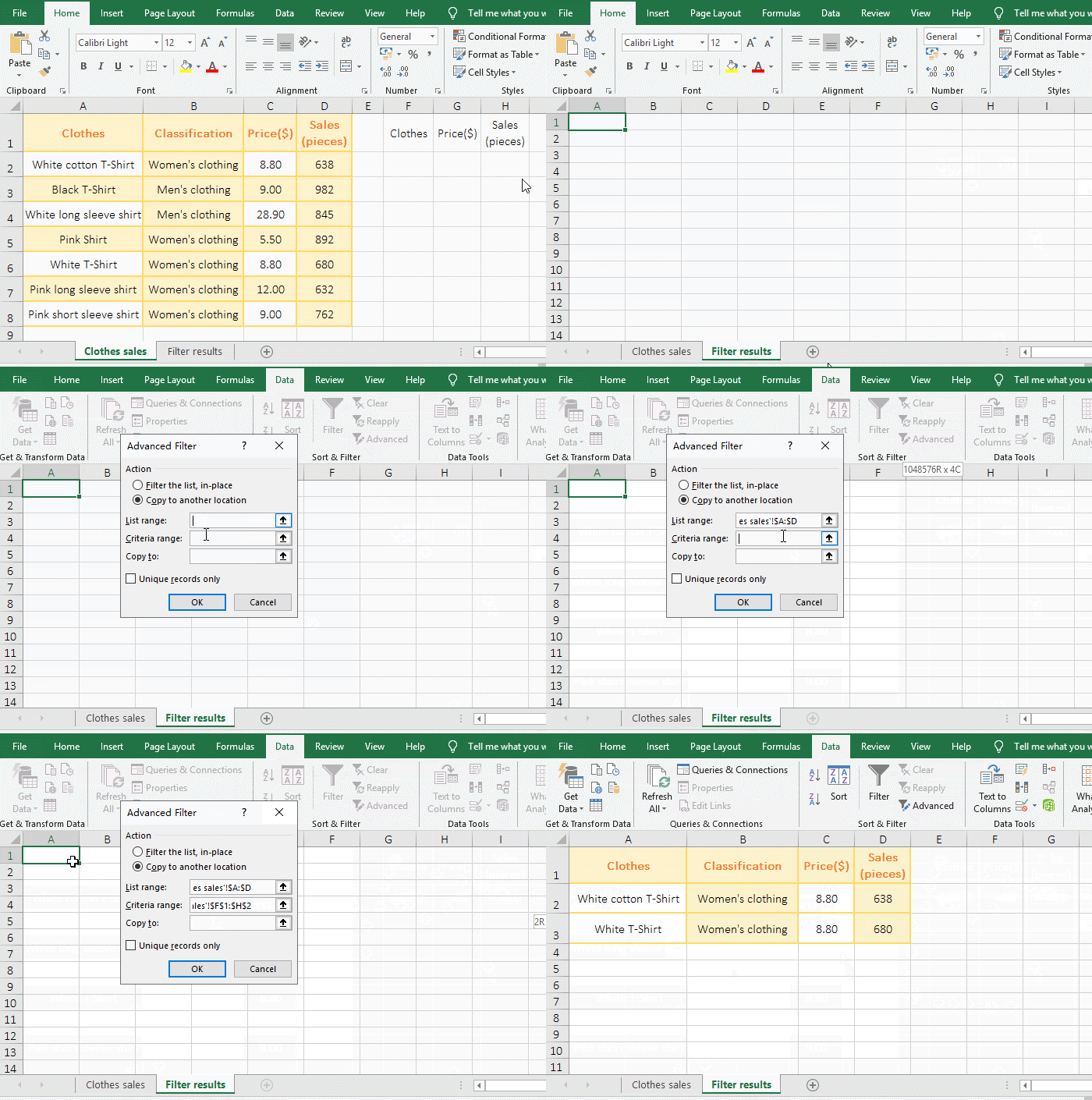
2. Advanced filtering settings.
A. Click the "Filter results" tab to switch to the worksheet, click the cell A1, hold down Alt, select "Data" tab, click "Advanced" to open the "Advanced Filter" dialog.
B. Select "Copy to another location", click the textbox to the right of "List range", position the cursor here, click the "Clothes sales" tab to switch to the worksheet, and select column A to column D, then "'Clothes sales'!$A:$D" is automatically entered into the "list range" textbox;
C. Then position the cursor to the right of the "Criteria range", Excel automatically switches back to the "Filter results" worksheet, click the "Clothes sales" tab again to switch the worksheet, and select F1:G2, then "'Clothes sales'!$F$1:$G$2" is automatically filled to the right of the "Criteria range";
D. Position the cursor to the right of "Copy to", click the cell A1, and "'Filter results'!$A$1" will be automatically filled in to the right of "Copy to"; check "Unique records only" and click "OK", then filter out two clothes that meet three criteria; the process steps, see screenshot in Figure 4:
Figure 4
III, How to modify and remove filter in excel
(I) How to modify filter in excel
1. If you want to change the two criteria to a criteria. Hold down Alt, press A and Q once, open the "Advanced Filter" dialog, select "Copy to another location", click the end of the text in the textbox to the right of "Criteria range", and select G1:G2, the reference criteria are change to $G$1:$G$2, check "Unique records only", click "OK" to filter all clothes with "Price" greater than or equal to $10; the operation steps are as shown in Figure 5:
Figure 5
2. When modifying the reference range, be sure to position the cursor at the end of the existing reference range(as in the demo, position the cursor at the end of the text in "Criteria range" textbox), otherwise the newly selected reference range will be inserted into the middle of the original reference range, the reference range is messed up. Also, if you previously selected "Copy to another locations" and "Unique records only", you will need to do it again.
(II) How to remove filter in excel
Select the "Data" tab, click "Clear"(or press Alt, press A and C respectively), the filter is cleared; the process steps, as shown in Figure 6:
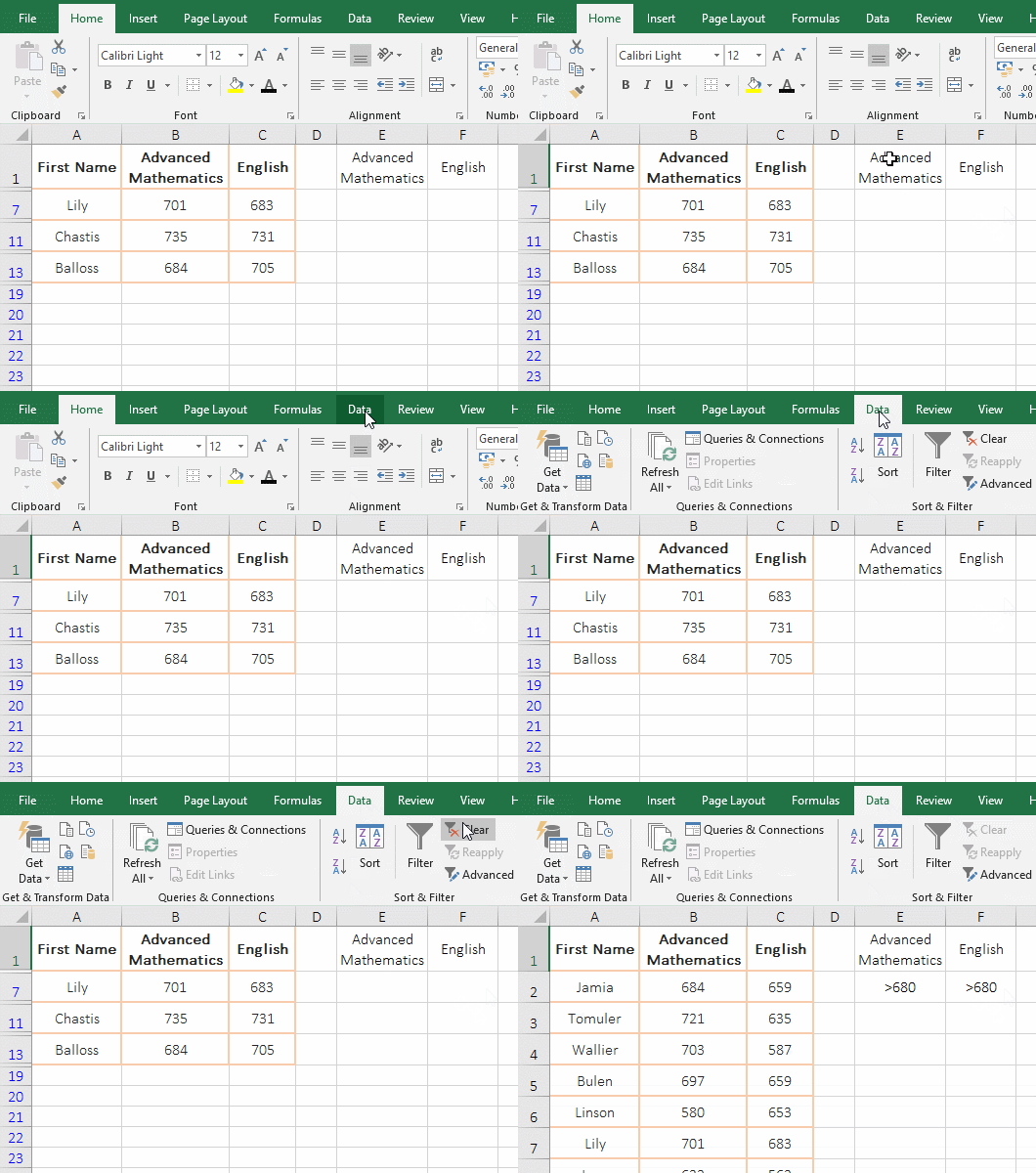
Figure 6
IV, Excel advanced filter extension application
(I) Not equal to empty, equal to empty and date as criteria(Excel advanced filter date range)
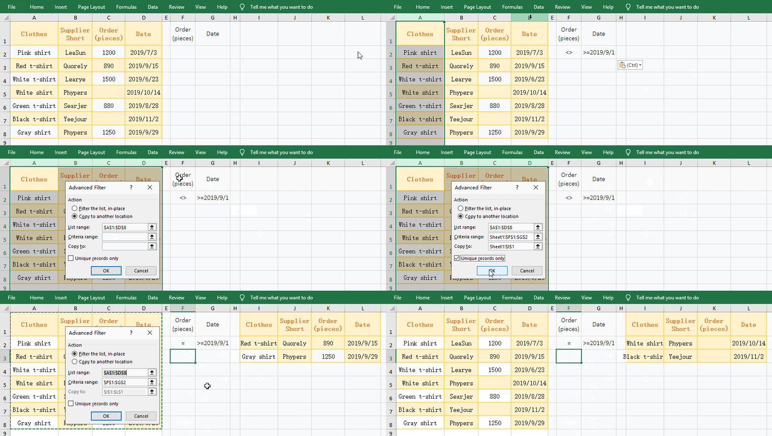
1. Preparation criteria. If you want to filter the "order quantity" is not empty and the date is greater than or equal to 2019-9-1, then filter the "order quantity" is empty and the date is greater than or equal to 2019-9-1. Enter "Order(pieces) and Date" in F1 and G1 respectively, enter <> in F2, select G2, and copy the criteria >=2019-9-1 to G2, the first criteria is ready. <> means not equal to empty, = means equal to empty.
2. Advanced filtering settings.
A. Click column A to select the first column, hold down Shift, and then click column number D to select the table. Hold Alt and press A and Q respectively to open the "Advanced Filter" dialog, select "Copy to another location", click the textbox to the right of "Criteria range" to position the cursor here, select F1:G2, position the cursor to the "Copy to" textbox, click I1(indicating that the filter result is copied to I1) , select "Unique records only", click "OK" to filter out the clothes that meet the first criteria.
B. Select F2, enter equal to =, press Enter, then press the shortcut keys Alt + A + Q to open the "Advanced Filter" dialog, select "Copy to another location" again and check "Unique records only", click "OK", then filter out the clothes that meet the second criteria; the operation process steps, see screenshot in Figure 7:
Figure 7
(II) Combining criteria with wildcards
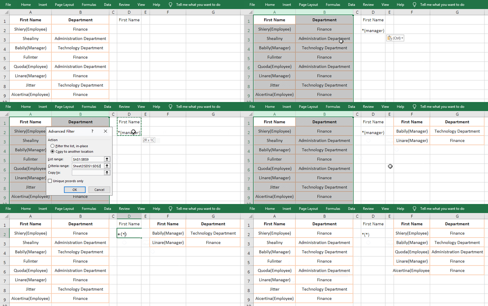
1. Preparation criteria. Suppose you want to filter employees with arbitrary characters before the parentheses and "manager" in parentheses and filter the annotated employees. Enter "First Name" in D1 and copy the criteria *(manager) to D2, the first criteria is ready. "*(manager)" means beginning with any one or more characters and containing "(manager)"; "*(*)" means starting with any one or more characters and having double brackets.
2. Advanced filtering settings.
A. Click column A to select the first column, press the left button and drag to column B, select the table, hold down Alt, press A and Q once, open the "Advanced Filter" dialog, and select "Copy to another location", click the "Criteria range" textbox to position the cursor inside, select the criteria D1: D2, position the cursor to the "Copy to" textbox, click F1, check "Unique records only", click "OK" to filter out the employees who meet the first criteria "*(manager)".
B. Select D2, change the criteria to *(*), and press Alt + A + Q to open the "Advanced Filter" dialog, select "Copy to another location", and check "Unique records only", click "OK" to filter out all employees who meet the second criteria *(*); the process steps are as shown in Figure 8:
Figure 8
Hint: If you want to the characters that are grouped by specifing a few characters on the right side of the brackets(such as four characters) and any characters in parentheses, the criteria can be written as: ????(*), a question mark represents a character in the criteria. If the text before the parentheses consists of any characters and the text in parentheses requires only four characters, the criteria can be written as *(????).
(III) Combining criteria with formula(Excel advanced filter formula)
1. Preparation criteria. If you want to filter the clothes whose "Classification" are "women's clothing", "Price" is greater than or equal to 8, and "Sales" is greater than or equal to 600. Double-click the cell F2 and copy the formula =(Classification="Women's clothing")*(price >= 8)*(sales >= 600) to F2, press Enter, return the name error #NAME?, leave it alone, the criteria are ready.
2. Advanced filtering settings. Click column A, select the first column, hold down Shift, click D column, select the table, hold down Alt, press A and Q respectively, open the "Advanced Filter" dialog, select "Copy to another location", click the "Criteria range" textbox to position the cursor inside, select F1:F2, position the cursor to the "Copy to" textbox, click G1, and then check "Unique records only", click "OK" to filter out the clothes that meet the three criteria; the operation steps are as shown in Figure 9:
Figure 9
Tip: Use the formula as the criteria, you can not write the field name, but you need to leave an empty cell on the formula. When the criteria are selected, you must select the formula and the empty cell above, otherwise an error will occur.
3. Formula description:
Formula =(Classification="Women's clothing")*(price >= 8)*(sales >= 600) consists of three criteria, the expression in each parenthese is a criteria, and the criteria and criteria are connected by an asterisk *, indicating the relationship "AND", that is, three criteria must be met at the same time. In addition, the formula can also be combined with the And function, then the above formula can be changed to =AND(Classification="Women's clothing", price >= 8, sales>=600).
Common criteria formulas:
1. The formula of filtering the data starting with the specified characters
If you filter clothes that start with "black" and sales between 700 and 900, the criteria formula can be written as follows: =(LEFT(product name,1)="black")*(sales >= 700)*(sales <= 900). Since the wildcard asterisk * cannot be used in the criteria formula, the first character of the "product name" is intercepted with LEFT(product name, 1).
2. The formula of filtering the data ending with the specified characters
If you want to filter clothes that end with the "T-shirt" and the price is above 90, the criteria formula can be written as follows: =(RIGHT(product name,2)="T-shirt")*(price > 90); RIGHT(product name,2)) is used to extract 2 characters from the right of Product Name.
-
Related Reading
- Excel Search function and SearchB usage(13 examples,
- 8 examples of Excel Match function, include it and S
- How to use offset function in excel, include it and
- How to use Excel small function and it and index, ma
- VLookUp in excel introduces step by step(10 examples
- How to use Excel address function(7 examples, with I
- How to find duplicate values in excel using vlookup(
- How to filter in excel(16 examples, with number,text
- How to use hlookup in excel(7 hlookup example, combi
- How to use excel Index function, include it and Matc
- Vlookup with if statement(use if/if{0,1} combination
- How to sort in excel(11 examples), include sort by c

