 Office > Excel > Excel 2019 > Content
How to remove duplicates in excel and find duplicates in rows or columns and mark with color
If you want to mark colors for duplicates(duplicate data) in excel, you can use conditional formatting; if you want to delete duplicate data, you can use excel remove duplicates and advanced filter; if you want to find(filter) two or more than two columns of the same data and the same data as one row, you need to use the formula
Excel can delete only one column of duplicates and the entire row of duplicates. To find data with two or more two columns and even one row, you need to use several function combinations, for example, using the IF + Sum + Value function combination.
I, How to find duplicates in exce with marking color(Highlight duplicates in excel)
(I) Marked with "Highlight Cell Rules"
1. Click the column number A, select the first column, select the "Home" tab, click "Conditional Formatting", select "Highlight Cell Rules → Duplicate Values" in the pop-up menu, open the "Duplicate Value" dialog, click "OK", then all the duplicate values in column A are marked with "Light Red Fill With Dark Red Text", the operation steps are as shown in Figure 1:
Figure 1
2. If you want to fill with another color, click the drop-down list box on the right side of the "Duplicate Value" dialog to select a color; if the required color is not met, select the last "Custom Format" to open the "Format Cells" dialog, select the "Fill" tab and choose a color.
Tip: Open the "Duplicate Value" dialog, you can use the shortcut keys Alt + H + L + H + D, the key method is: hold down Alt and press H, L, H and D respectively.
(II) Mark with "Format only unique and duplicate values"
1. Click the column number A and select the A column, te current tab is "Home", click "Conditional Format", select "New Rule" in the pop-up menu, open "New Formatting Rule" dialog, Select "Format only unique and duplicate values", select "duplicate" for "Format all", click "Format", open the "Format Cells" dialog, select the "Fill" tab, select a color(such as "Green" ), click "OK" twice, then all duplicates in column A are marked in green; the operation process is shown in Figure 2:
Figure2
2. open the "New Formatting Rule" dialog can also use the shortcut keys Alt + H + L + N, the button method is: hold down Alt, press H, L and N in turn.
Hint: This method can only mark duplicate data in one column, not data that is repeated in one row.
(III) Method of removing the color of the mark
1. Select column A, the current tab is "Home", click "Conditional Formatting", select "Clear Rules → Clear rules from selected cell" in the pop-up menu, then all the color markers in column A are cleared. Operation process steps, as shown in Figure 3:
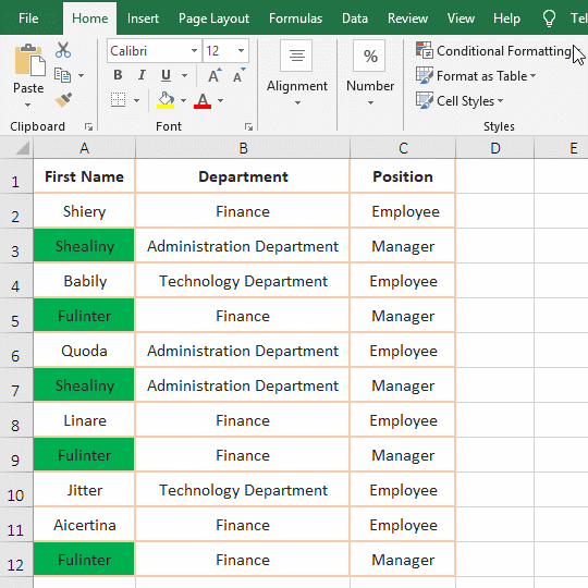
Figure 3
2. Press the shortcut keys Alt+ H + L + C + S to clear the mark color of the selected cells. The key press method is: hold down Alt and press H, L, C and S respectively. If you want to clear the color mark of the entire table, you can press the shortcut keys Alt+ H + L + C + E, the key method is the same as above.
II, How to remove duplicates in excel(Merges duplicate data)
(I) How to delete with "Remove Duplicates"
1. How to remove duplicate rows in excel? Select one of the cells in the table, select the "Data" tab, click "Remove Duplicates", open the "Remove Duplicates" dialog, list three fields, the checked checkbox are counted the field into the duplicate, keep check all fields in the table to delete the duplicate rows, click "OK", a small dialog pops up prompting "3 duplicate values found and remove; 8 unique values remain.", click "OK", then the three duplicate rows (rows 7, 9 and 12) are deleted, the operation process steps, see screenshot in Figure 4:
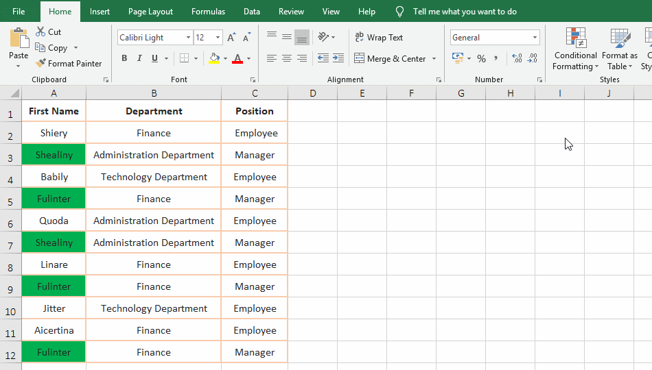
Figure 4
2. Excel remove duplicates in column. Click column Number A to select column A, hold down Alt, press A and then M, open the "Remove Duplicate Warning" dialog, select "Continue with the crrent selection", and click "Remove Duplicates" to open "Remove Deduplicates" dialog, click "OK", click "OK" in the pop-up dialog, only the duplicates in column A are deleted, and the data of the other columns corresponding to column A are not deleted; the steps are as shown in Figure 5:
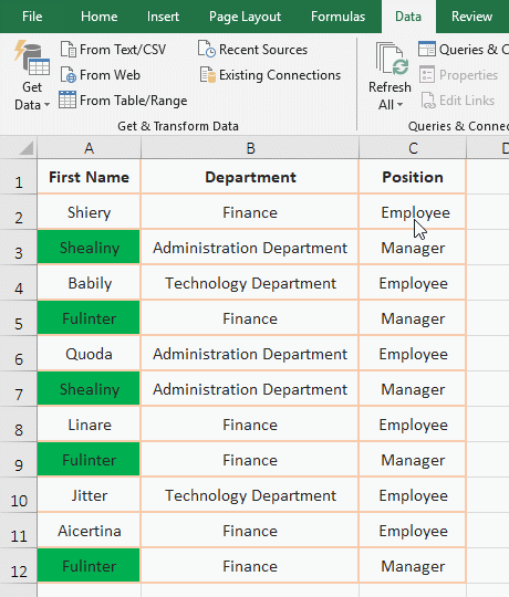
Figure 5
Hint: If you select "Extend the selection", it will delete the duplicate of one row, which is equivalent to the operation of Figure 4.
3. Duplicate items in two columns, deleting duplicates in a row. Select one of the cells in the table, hold down Alt, press A and M respectively, open the "Remove Duplicates" dialog, click "First Name" to uncheck it, only check "Department and Position", click "OK" , pop-up the dialog prompts 5 duplicate values are removed, click "OK", then the values duplicated in both columns B and C are deleted, respectively, rows 7, 9 and 12; as shown in Figure 6:
Figure 6
Tip: If you check more than two fields at the same time, only the checked fields are the same, and delete one row instead of just the selected one.
(II) How to delete with "Advanced filter"
1. Click column A to select column A, and hold down the left button to drag to column C, select the table, select the "Data" tab, click "Advanced" in the upper right corner of "Sort & Filter" to open "Advanced Filter" dialog, click "Unique records only" to check it, click "OK", then the duplicate items (repeated rows) is deleted; the operation process steps, see screenshot in Figure 7:
Figure 7
2. Open the "Advanced Filter" dialog,you can press the shortcut keys Alt + A + Q. The button method is: hold down Alt and press A and Q one time.
III, How to formula to find duplicates in excel
(I) Excel find duplicates in column
1. If you want to find out if there are duplicate items in the "First Name" of the employee in column A. Double-click the cell D2, copy the formula =IF(COUNTIF(A$2:A$12,A2)>1,"Duplicate","") to D2, press Enter, return empty; select D2, move the mouse to the cell fill handle in the lower right corner of D2, after the mouse changes to the bold black plus sign, double-click the left button to mark the remaining rows as duplicates; the operation steps are as shown in Figure 8:
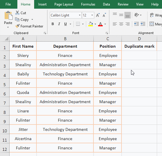
Figure 8
2. The formula =IF(COUNTIF(A$2:A$12,A2)>1,"Duplicate","") description:
A. A2 means that the column and row are relative references, when dragging down, A2 will automatically change to A3, A4, ...; when dragged to the right, A2 will automatically change to B2, C2, ....
B. A$2 means relative reference to the column, absolute reference to the row, when dragging down, A2 will not become A3, A4, ...; but when dragging to the right, A2 will automatically become B2, C2, ...; A$12 and A$2 are a meaning. The effect is of A$2:A$12: no matter how you drag down, always make sure to count in A2:A12.
C. COUNTIF(A$2:A$12,A2)>1 is the criteria of If, when the formula is in D2, the number of A2 in A2 to A11 is counted; when the formula is in D3, it becomes COUNTIF(A$2: A$12,A3)>1, which counts the number of A3 in A2 to A12, and so on.
D. Since the result of COUNTIF(A$2:A$12, A2) is 1,1>1 is not true, so the third argument of If is returned, that is, it returns null. The COUNTIF(A$2:A$12,A3) has a statistical result of 2, 2>1, so the second argument of If is returned, that is, returns "Duplicate".
Hint: If you want to count the duplicates two or more than two culumns, you can't write the formula =IF(COUNTIFS(A$2:A$12,A2,B$2:B$12)>1,"Duplicate",""), because this is to count the duplicates in each column, instead of counting the duplicates of column A first, and then counting the duplicates in column B corresponding to column A.
(II) Find duplicates in two columns in excel(or excel find duplicate rows)
1. Find two columns with the same duplicate at the same time, for example: A3 repeats with A7 and B3 repeats with B7. Double-click the cell D2 and copy the formula =IF(SUM(--(A$2:A$12&B$2:B$12=A2&B2))>1,"Duplicate","") to D2, press Ctrl + Shift + Enter , return empty, double-click the cell fill handle of D2, return the duplicate mark result of the remaining rows; the operation process steps, see screenshot in Figure 9:
Figure 9
2. Formula =IF(SUM(--(A$2:A$12&B$2:B$12=A2&B2))>1,"Duplicate","") explanation:
A. The formula is an array formula, so press Ctrl + Shift + Enter.
B. A$2:A$12 returns the value in A2:A12 as an array, and B$2:B$12 returns the value in B2:B11 as an array. A$2:A$12&B$2:B$12 connects the value returned by A2:A12 with the value returned by B2:B12, for example, returns A2 and B2 for the first time, A2&B2 for "ShieryFinance", and returns A3 and B3 for the second time, A3&B3 is "ShealinyAdministration Department", and so on, and finally returns an array of A columns connect B columns.
C. Then A$2:A$12&B$2:B$12=A2&B2 becomes {"ShieryFinance"; "ShealinyAdministration Department"; ...;"FulinterFinance"}=A2&B2, then, the first time, takes the first element of the array "ShieryFinance" and A2&B2 (ie "ShieryFinance") compares, because they are equal, it returns True; the second time takes the second element of the array "ShealinyAdministration Department" and A2&B2 compares, because they are not equal, so return False, the other and so on, and finally returns {TRUE;FALSE;FALSE;FALSE;FALSE;FALSE;FALSE;FALSE;FALSE;FALSE}.
D. Then SUM(--(A$2:A$12&B$2:B$12=A2&B2)) becomes SUM(--({TRUE;FALSE;FALSE;FALSE;FALSE;FALSE;FALSE;FALSE;FALSE;FALSE}) ), further calculations, convert the logical values in the array into numbers and add them together, the result is 1, The function of -- is to convert the text or logical values into numbers for calculation, which is equivalent to the Value function. The Sum function is used here to count the number of rows in which the corresponding rows are the same.
E. The formula becomes =IF(1>1,"Duplicate",""), 1>1 is the criteria of If, since it does not hold, the third argument of If is returned ""(empty).
3. Find duplicates that are repeated throughout the entire row. Simply connect each column with & and the formula can be written like this: =IF(SUM(--(A$2:A$12&B$2:B$12&C$2:C$12=A2&B2&C2))>1,"Duplicate","").
4. Change the above formula to =SUM(--($A$1:$A$12&$B$1:$B$12&$C$1:$C$12=A1&B1&C1))>1, which can mark the duplicates in row with a color, the operation process steps, as shown in Figure 10:
Figure 10
Operation procedure step description: Click column number A to select column A, drag to column C, select the table, hold down Alt, press H, L and N once, open the "New Format Rule" dialog, select "Use a formula to determine which cells to format", copy the formula =SUM(--($A$1:$A$12&$B$1:$B$12&$C$1:$C$12=A1&B1&C1))>1 to the textbox under "Form values where this formula is true", click "Format" to open the "Format Cells" dialog, select the "Fill" tab, select "Green", click "OK" twice, then the duplicates in column A are marked with green, double-click B7, enter 0, and the color of markers of A7 and A3 is removed, indicating that only all the fields in a row are the same to mark green.
Hint: Since the formula combines the data of the corresponding row of each column, although only the duplicate data of column A is marked, all the ones marked are repeated.
(III) The first duplicate item is marked 1, and the second item is marked with a value greater than 1
1. Also take the example of finding the same data for two columns or the entire row. Double-click the cell D2, copy the formula =SUM(--($A$2:A2&$B$2:B2=A2&B2)) to D2, press Enter, return to 1, double-click the cell fill handle of D2, and return the counted result of the remaining rows, the value greater than 1 is a duplicate; the operation process steps, see screenshot in Figure 11:
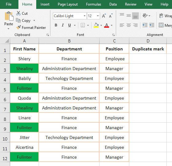
Figure 11
2. The formula =SUM(--(A$2:A2&B$2:B2=A2&B2)) description:
A. A$2:A2 is used to count to the current row. When the formula is in D2, A$2:A2 returns A2, B$2:B2 returns B2, A$2:A2&B$2:B2=A2&B2 becomes A2&B2=A2&B2, equation holds, returns True, the formula becomes =SUM(--(TRUE)), and the further calculation becomes =SUM(1), so returns 1. The function of -- has been introduced above.
B. When the formula is in D3, the formula becomes =SUM(--(A$2:A3&B$2:B3=A3&B3)), and the formula is the same as "(II) Find duplicates in two columns in excel(or excel find duplicate rows)".
-
Related Reading
- Excel CountA and CountBlank function usage examples(
- 8 examples of Excel Match function, include it and S
- How to use offset function in excel, include it and
- Excel SumProduct function(multiple criteria, with if
- Excel Countifs formula examples, include with And, O
- Excel left function usage(8 examples, with Sum+Value
- How to use Average function in excel(combine with if
- How to use advanced filter in excel(7 examples, mult
- How to use Excel address function(7 examples, with I
- How to filter in excel(16 examples, with number,text
- Excel SumIf function with ?/*, Average and array mul
- How to use Excel subtotal function(combine it with O