How to use Excel Right function and RightB(8 examples, with Find, Len, Trim in formula)

Both the Right function and RightB function are used to extract the specified number of characters starting from the first character on the right side of the text in Excel; but they differ: the Right function is in characters, it counts a full-width (such as "Chinese, Japanese characters and Korean characters") and a half-width (such as "number and letter") as one character; the RightB function is counted in bytes, which counts full-width characters as two bytes and half-width characters as one byte when you have enabled the editing of a language that supports DBCS and then set it as the default language. In addition, similar to the Right and RightB functions are Left, LeftB and Mid, and MiddB functions.

The Right and RightB function are often used in combination with the Len, Trim, Left and Find function. The Right + Len + Find combination can be used to intercept any specified characters from the right side of the text and intercept the specified characters with a different length of text and after any specified character; the Right + Trim function combination implementation first remove spaces before intercepting.

I, Excel Right function and RightB function syntax

1. Right function expression: RIGHT(Text, [Num_Chars])

2. RightB function expression: RIGHTB(Text, [Num_Bytes])

3. Description:

A. The Right and RightB functions are used to extract characters of the specified length from the right, but there are differences between them: the Right function counts all characters(such as "Chinese, Japanese characters and Korean characters") and half-width (such as "numbers and letters") as one character; the RightB function counts full-width characters as 2 bytes and half-width characters as 1 byte.

B. Num_Chars is optional. If omitted, the Right function extracts 1 character by default; Num_Chars must be greater than or equal to 0, otherwise it will return the value error #VALUE!; If Num_Chars is greater than the length of text, the Right function will return all text.

C. Num_Bytes is also optional. If omitted, RightB function extracts 1 byte by default; Num_Bytes must be greater than or equal to 0, otherwise it will return value error #VALUE!; If Num_Bytes is greater than the total number of bytes of text, RightB function will return all text.

II, How to use Right function in excel

(I) Extract a specified string from text consisting of numbers, letters characters

1. Double-click the cell B1, copy the formula =RIGHT(A1,4) to B1, press Enter, return t8.8; select B1, move the mouse to the cell fill handle in the lower right corner of B1, double-click Left button after the mouse change to the bold black plus, the 4 characters in A2 and A3 is also extracted from the right; the operation steps, as shown in Figure 1:

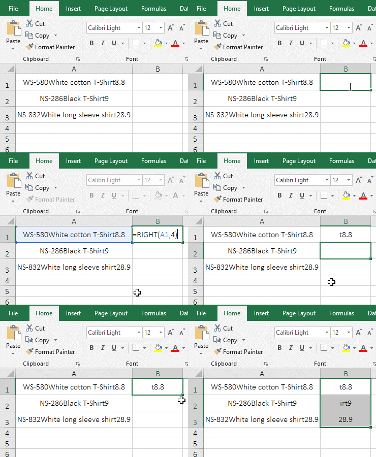
Figure 1

2. Formula description:

A1 is the Text to extract the character, and 4 is the Num_Chars in the formula =RIGHT(A1,4). The formula means: 4 characters are extracted from the first character on the right side of A1, which is exactly t8.8.

(II) Num_Chars is omitted and must be greater than or equal to 0

1. Double-click the cell B1, copy the formula =RIGHT(A1) to B1, press Enter, return to 8; double-click B1, enter a comma(,) after A1, press Enter, return empty text; double-click B1, after the comma Enter 0, press Enter, return empty text; double-click B1 again, change 0 to -1, press Enter, return value error #VALUE!; operation process steps, as shown in Figure 2:

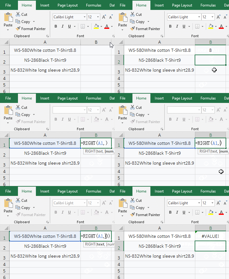
Figure 2

2. Formula description:

A. The argument Num_Chars is omitted in the formula = RIGHT(A1), and one character is extracted by default, so 8 is returned.

B. The both formula =RIGHT(A1,) and =RIGHT(A1,0) return empty text, indicating that when the Num_Chars is omitted, the comma cannot be added after the first parameter; if the comma is added, the Num_Chars is set to 0.

C. Formula =RIGHT(A1,-1) set the Num_Chars to -1, since the Right function requires that the extracted characters must be greater than or equal to 0, the return value is incorrect.

(III) Right + Len returns all text

1. Double-click the cell B1, copy the formula =RIGHT(A1,LEN(A1)) to B1, press Enter, return all the text in A1; double-click B1, change LEN(A1) to LEN(A1)+1 , press Enter, also return all the text in A1; the operation process steps, as shown in Figure 3:

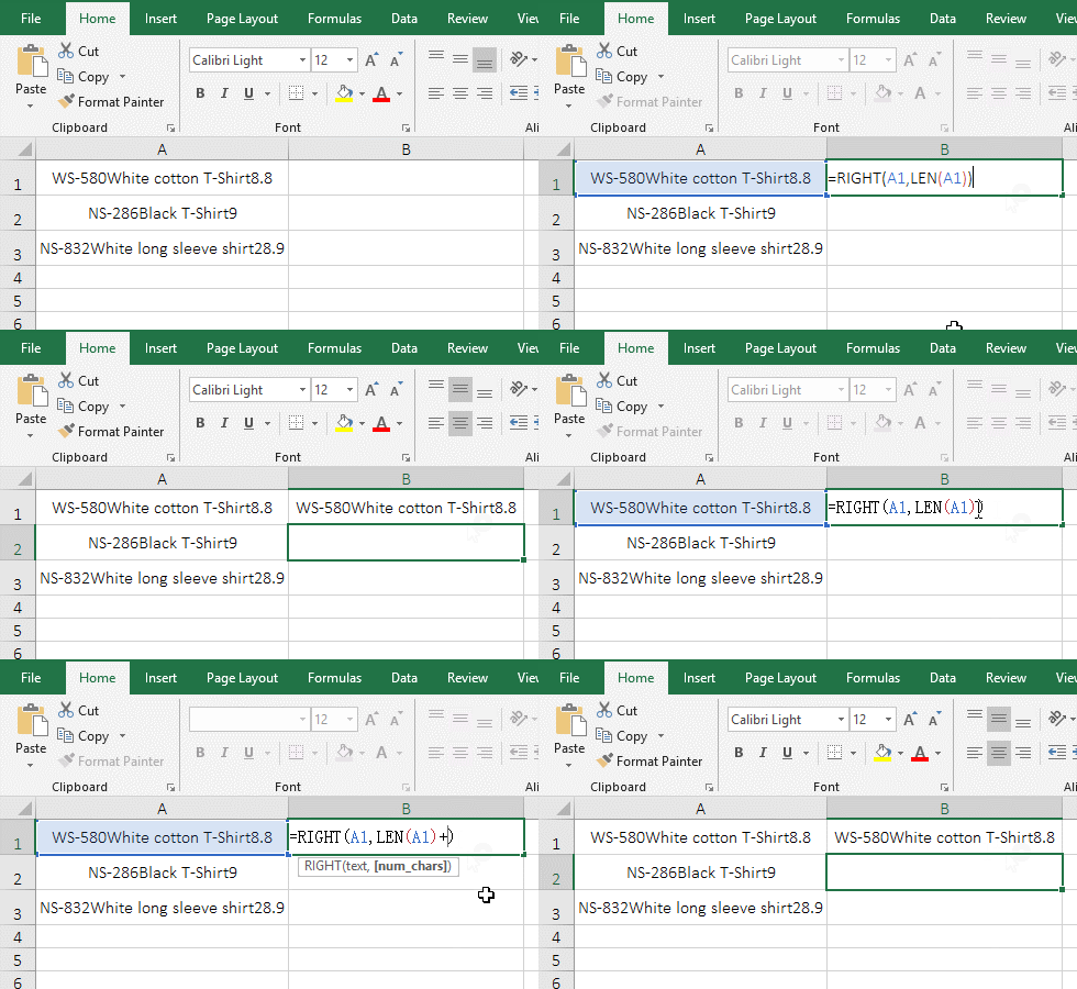
Figure 3

2. Formula description:

A. returns the text length of A1 with LEN(A1) for the first time in the formula =RIGHT(A1,LEN(A1)), then use Right to intercept all the text in A1 from the right.

B. The Num_Chars LEN(A1)+1 is greater than the length of all texts of A1 in the Formula =RIGHT(A1,LEN(A1)+1), but only all the texts in A1 are returned, indicating that the Num_Chars is greater than the length of the text, the Right function extracts only all the text.

III, How to use RightB function in excel

(I) Extract any specified characters from the right side of text

1. Double-click the cell B1, copy the formula =RIGHTB(A1,3) to B1, press Enter, return to "8.8"; the operation steps are as shown in Figure 4:

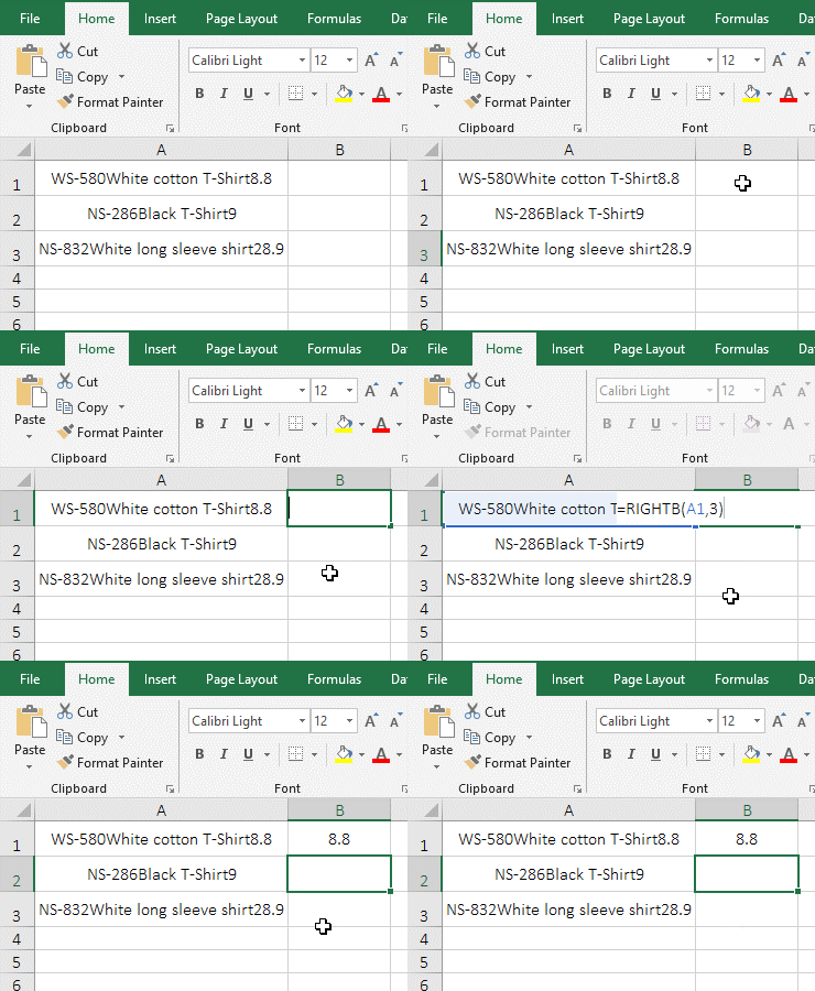
Figure 4

2. Formula description:

A1 is the argument Text, 3 is the Num_Bytes in the formula =RIGHTB(A1,3), The formula means: extracts 3-byte characters from the first character on the right.

(II) RightB + LenB returns all text

1. Double-click the cell B1, copy the formula =RIGHTB(A1,LENB(A1)) to B1, press Enter, return all the text in A1; double-click B1 to change LENB(A1) to LENB(A1)+1 , press Enter, also return all the text in A1; the operation process steps, as shown in Figure 5:

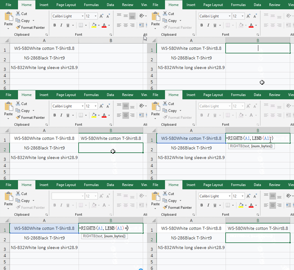
Figure 5

2. Formula description:

A. LENB(A1) is used to return the total number of bytes of all text in A1 in the formula =RIGHTB(A1,LENB(A1)), the result is 29; the formula becomes =RIGHTB(A1,29), and returns 29 bytes of text from the first character on the right, which returns all the text in A1.

B. LENB(A1)+1 is greater than the total number of bytes of all text in A1 in the formula =RIGHTB(A1,LENB(A1)+1), but still only returns all the text in A1, indicating that when the number of extracted bytes is greater than the total number of bytes of all text, the RightB function returns only all text. The reason for adding 1 is to ensure that the number of extracted bytes is long enough.

IV, The application examples of Excel Right function and of RightB function

(I) Right and Find function in excel: Right + Len + Find function combination to intercept any specified character from the right

1. If you want to intercept the "Clothing Name" on the right side of "WS-580White cotton T-Shirt". Double-click the cell B1, copy the formula =RIGHT(A1,LEN(A1)-FIND("White",A1)+1) to B1, press Enter, return to "White cotton T-Shirt"; operation process Steps, as shown in Figure 6:

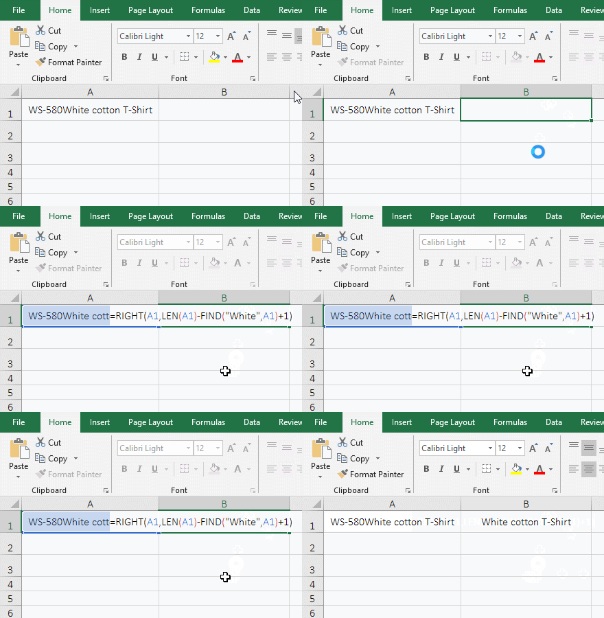
Figure 6

2. Formula =RIGHT(A1,LEN(A1)-FIND("White",A1)+1) explanation:

A. FIND("White",A1) returns the position of the "White" in A1, the result is 7; the "White" is the first word of the text to be intercepted from the left.

B. LEN(A1) returns the length of text in A1, the result is 26.

C. LEN(A1)-FIND("White",A1)+1 is used to calculate the number of characters to be intercepted. Substituting the above values ??into 26 - 7 + 1, the result is 20.

D. The formula becomes =RIGHT(A1,200), and finally the Right function is used to cut 20 characters from the first character on the right side, which is exactly the "Clothing Name" in A1.

In addition, you can also use the RightB + LenB + FindB to achieve the same function, the formula can be written like this: =RIGHTB(A1,LENB(A1)-FINDB("White",A1)+1), each function in the formula counts full-width as 2 bytes and half-width as 1 byte.

(II) Right + Len + Find function combination to intercept tha all characters after a specified character of a different length of text

1. If you want to intercept all the numbers after "c" in column A. Double-click the cell B2, copy the formula =RIGHT(A2,LEN(A2)-FIND("c",A2)) to B2, press Enter, return to 98643; the operation steps are as shown in Figure 7:

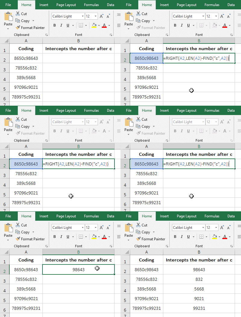
Figure 7

2. Formula =RIGHT(A2,LEN(A2)-FIND("c",A2)) explanation:

The formula and the above formula =RIGHT(A1,LEN(A1)-FIND("White",A1)+1) is a meaning, if you want to intercept with "c", you need to add 1 again, that is =RIGHT(A2,LEN(A2)-FIND("c",A2)+1).

(III) Excel right trim: Right and Trim function combination implementation first remove spaces before intercepting

1. if the text to be intercepted some of the front with spaces, some after with spaces and some without spaces. Select Cell B2, enter the formula =right(A2,5), press Enter, return 8643, and return the remaining interception results by double-clicking the cell fill handle in lower right of B2. Double-click C2, copy the formula =RIGHT(TRIM(A2),5) to C2, press Enter, return 98643. the procedure steps, as shown in Figure 8:

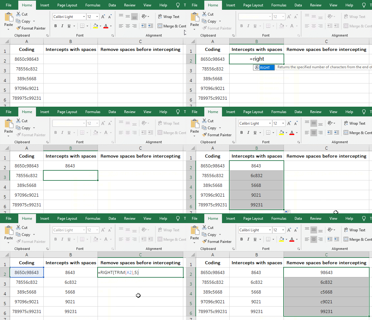
Figure 8

2. Formula description: 

A. Formula =RIGHT(A2,5) and =RIGHT(TRIM(A2),5) are different: the former does not remove the space before the interception, the latter first remove the space before the interception; for example, 8643 in B2 is less 9, and 98643 in C2 is the correct result.

B. TRIM(A2) is used to remove spaces before and after the text in A2.