How to use Excel Trim function(6 examples, with leading,trailing,stubborn spaces and Left)

The Trim function is used to remove the leading spaces and trailing spaces and spaces between characters in Excel, but when you remove spaces between characters, it does not remove all spaces, but leaves a space; if you want to remove All spaces between characters, you need to use the Substitute function.

When deleting spaces in Excel, you often encounter some stubborn spaces. You can't remove them with the Trim or Clean function. You need to replace them with the Substitute function. If you still cannot remove them with the Substitute function, you need to combine them with the Left, Right, and Code functions. In order to remove the space. In addition, if the number with spaces will not be able to return the correct result, in this case you need to use the TRIM function to remove the space and then sum.

I, The syntax of the Excel Trim function

1. Expression: TRIM(Text)

2. Description:

Text is the text to remove the space; the Trim function removes all leading spaces and trailing spaces text, but if you want to remove the space between the text, it will not remove all the spaces, but leave one.

II, The examples of Excel Trim spaces

(I) Trim leading spaces and Trim trailing spaces in excel

If you want to remove all the spaces before and after the text "  Excel function tutorial  ". Double-click the cell A1, copy the formula =TRIM("  Excel function tutorial  ") to A1, press Enter, return to "Excel function tutorial"; the current cell is align left, the text is to the left, and the left space is removed; click "Align Right" icon, the text is on the right, and the space on the right is removed. The operation steps are as shown in Figure 1:

Figure 1

(II) Examples of removing spaces between characters

1. If you want to remove the space in the text "Excel   Function   Tutorial". Select the cell B1, enter the formula =TRIM(A1), press Enter, and return to the "Excel Function Tutorial". Double-click B2, copy the formula =SUBSTITUTE(A1," ","") to B2, press Enter, return to "ExcelFunctionTutorial". The operation steps are as shown in Figure 2:

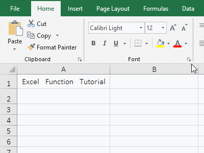
Figure 2

2. Formula description:

A. The formula =TRIM(A1) is not completely removed the spaces in the text in A1, and a space is left in the space.

B. The formula =SUBSTITUTE(A1," ","") removes all the spaces in the text in A1; Substitute function is a replacement character function, which means here, replaces all spaces with the empty text "".

III, How to trim spaces in excel: The stubborn spaces removal method(Trim function does not work solution)

(I) The space that can be removed can be copied

1. Double-click the cell E2, enter the formula =TRIM(A2), press Enter, the space in A2 is not removed; double-click E2, change TRIM to CLEAN, press Enter, the space in A2 is still there; double click E2 again, change CLEAN(A2) to SUBSTITUTE(A2," ",""), press Enter, the space in A2 is still there; double-click A2, select the space with the mouse, press Ctrl + C to copy, then double-click E2 , select the replaced space " ", press Ctrl + V paste, press Enter, the space in A2 is replaced; the operation steps, as shown in Figure 3:

Figure 3

2. Formula description:

A. The formula =TRIM(A2) and =CLEAN(A2) can not remove the space in A2, indicating that the space is not a normal space and non-printing characters generated by the Space on the keyboard; Clean function is used to remove non-printing characters.

B. The replaced character " " in the formula =SUBSTITUTE(A2, " ", ""), when you enter by Space on the keyboard, you cannot replace the space in A2. Only copy the space in A2 to the replaced character, the space in A2 are replaced.

Tip: If you still can't remove the space with the Substitute function, you can press Ctrl + H to open the "Find and Replace" window, copy the characters that cannot be replaced to the input box to the right of "Find What", click "Replace All" Can be removed.

(II) Spaces that cannot be removed cannot be copied

1. First check the ASCII code of the space; double-click the cell B1, copy the formula =CODE(LEFT(A1)) to B1, press Enter, and return to 63. Then replace the space with the ASCII code 63 that has been returned as a condition; double-click B2, copy the formula =SUBSTITUTE(A1,IF(CODE(LEFT(A1))=63,LEFT(A1)),"") to B2, Press Enter, all the spaces in front of text in A1 are removed, A1 has been set to center, the text is not centered because there is a space on the left, and the text in B2 is already centered, indicating that the space is removed; the operation steps, as shown in Figure 4:

Figure 4

2. Formula description:

A. LEFT(A1) is used to intercept a character from the left side of the text in A1 in the formula =CODE(LEFT(A1)), and then use the Code function to return the ASCII code of the intercepted character. The result is 63.

B. IF(CODE(LEFT(A1))=63,LEFT (A1)) is used to return a space that cannot be removed in the formula =SUBSTITUTE (A1,IF(CODE(LEFT(A1))= 63,LEFT(A1)),""), meaning: if the ASCII code of the space that has been replaced from the left of the text in A1 is equal to 63, the space is returned; CODE(LEFT(A1))=63 is the condition of If, 63 has been returned the ASCII code of the space in the cell B1; replaces the space whose ASCII code is 63 in A1 with the empty text("") finally.

IV, The extended application examples of Excel Trim function

(I) Excel Left Trim function combination intercepts after removing the spaces

1. If you want to extract the numbers in column A. Double-click the cell B1, copy the formula =LEFT(A1,3) to B1, press Enter, return empty text; double-click B1, add Trim() to A1, press Enter, return to 2.5; select B1, move the mouse to the cell fill handle in the lower right corner of B1, after the mouse becomes the bold black plus, double-click the left button to intercept the number of the remaining cells; the operation steps are as shown in Figure 5:

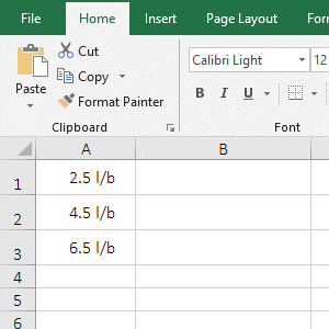
Figure 5

2. Formula =LEFT(TRIM(A1),3) description:

A. TRIM(A1) is used to remove the space to the left of "   2.5 l/b" in A1, it returns "2.5 l/b".

B. The formula becomes =LEFT ("2.5 l/b", 3), and intercepts finally 3 characters with Left function from the first character on the left, just cuts the number.

(II) Sum + Trim function combination adds the values with spaces

1. If the sum of sales is required, the value in the sales column is text with a space in front. Double-click the cell D9, enter the formula =SUM(D2:D8), press Enter, return 0; double-click D9, add TRIM() to D2:D8, press Ctrl + Shift + Enter, still return 0; double-click D9 again, enter -- before the TRIM, press Ctrl + Shift + Enter, return the summation result 5,028; the operation steps, as shown in Figure 6:

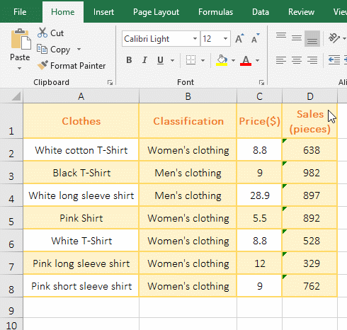
Figure 6

2. Formula =SUM(--TRIM(D2:D8)) explanation:

A. The formula =SUM(--TRIM(D2:D8)) is an array formula, so you need to press Ctrl + Shift + Enter; D2:D8 returns all the values in D2 to D8 as an array.

B. Then TRIM (D2:D8) becomes TRIM({" 638";" 982";" 897";" 892";" 528";" 329";" 762"}), then, the first element " 638" is taken from the array, and its space is removed for the first time; the second element " 982" is taken from the array, and its space is removed for the second time; the others and so on, and returns finally {"638";"982";"897";"892";"528";"329";"762"}.

C. Then the formula becomes =SUM(--{"638";"982";"897";"892";"528";"329";"762"}), further calculations, the elements in the array are converted from character to numeric, -- for converting characters to numeric values, which is equivalent to the Value function.

D. The formula is further changed to =SUM({638;982;897;892;528;329;762}), and adds finally all the elements in the array.

Tip: Since the number in D2:D8 is text type, when copying the formula to D9 and after pressing Enter, if you double-click D9 again, the formula will be displayed, press Enter, you can't sum again, because the format of D9 is changed to text type automatically, to solve this problem, you need to set the format of D9 to "value", the method: Pressing Ctrl + 1, open the "Format Cells" window, select "Number" Tab, then select "Number" on the left, if you do not want to keep the number of decimal places, set the "Decimal Places" to 0, and click finally "OK".