How to use Excel find function(9 examples, include find if,mid,sum combination)

The Find function is used to find the position of the specified text in the text of the search text in Excel. The FindB function has the same function as the Find function, except that the Find function counts both full-width characters(such as Chinese characters, Japanese characters and Korean characters) and half-width characters(such as numbers and letters) as one character, and the FindB function counts the full-width character as two bytes and the half-width character as one byte when you have enabled the editing of a language that supports DBCS and then set it as the default language.

The Find function and the FindB function are often combined with functions such as If, Sum, Mid, Left, and IsNumber in everyday applications, . For example, the combination of Mid + Find(or FindB) implements the interception of characters from any specified character. If + IsNumber + Find combination Implement dynamic lookups, and Sum + IsNumber + Find combines to find multiple values at once.

I, Excel Find function and FindB function syntax

1. Find function expression: FIND(Find_Text,Within_Text,[Start_Num])

2. FindB function expression: FINDB(Find_Text,Within_Text,[Start_Num])

3. Description:

A. Find function counts full-width characters(such as Chinese characters, Japanese characters and Korean characters) and half-width characters(such as numbers and letters) as one character. The FindB function counts full-width characters as two bytes and half-width characters as one byte. The Find and FindB function are case-sensitive and do not allow wildcards; if you want to ignore case and allow wildcards, you can only use the Search or SearchB function.

B. If Find_Text is empty text (""), the default position 1 of the first character is returned; Find_Text cannot contain any wildcard characters, such as question marks(?) or asterisks(*).

C. Start_Num is optional. If omitted, the default search starts from the first character; Start_Num is less than or equal to 0 or greater than or equal to the length of Within_Text, and both Find and FindB return value error #VALUE!.

D. If the Find_Text is not found in Within_Text, the value error #VALUE! is also returned.

II, How to use find function in excel(The use examples of Excel Find function)

(I) Find short text and omit the starting position of the search

1. If you want to find the position of lb in "1850lb". Double-click the cell E2, copy the formula =FIND("lb",D2) to E2, press Enter, return to 5; double-click E2 again, enter the comma after D2, press Enter, return value error #VALUE!; operation steps, as shown in Figure 1:

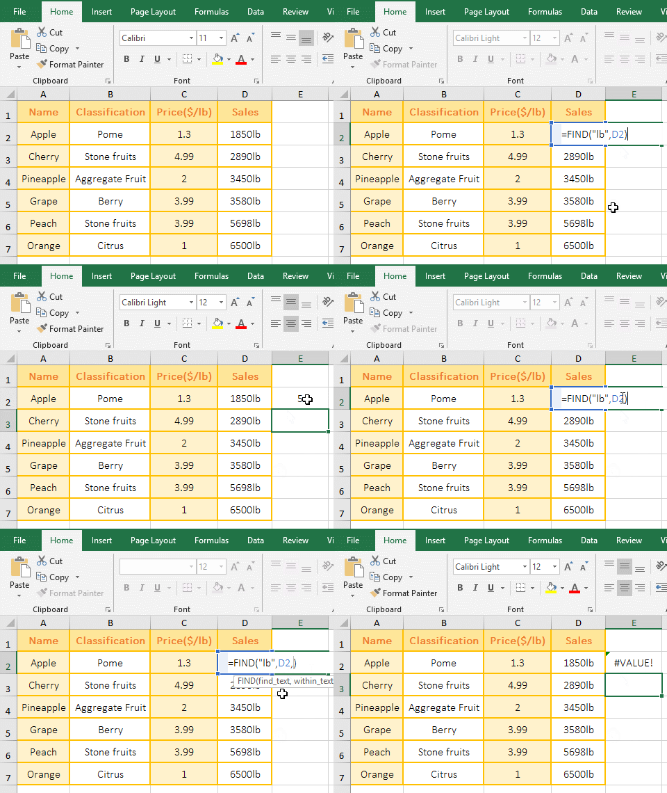
Figure 1

2."lb" is the Find_Text, D2 is the Within_Text in the formula =FIND("lb",D2), the formula omits the last argument Start_Num, it finds from the first character by default. In addition, the formula =FIND("lb",D2,) returns an error value, indicating that when Start_Num is omitted, the comma cannot be added after the second argument.

(II) Case sensitive and do not allow wildcards

1. If you want to find the case E in the "Excel tutorial". Double-click the cell B1, copy the formula =FIND("E",A1) to B1, press Enter to return to 1; double-click B2, copy the formula =FIND("E",A1) to B2, and change the capital E to lowercase e, press Enter, return 4; double-click B2 again, enter * after e, press Enter, return value error #VALUE!; operation process steps, as shown in Figure 2:

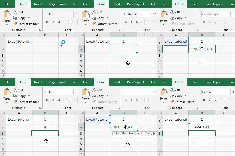
Figure 2

2. Formula description:

A. =FIND("E",A1) returns the position 1 of the uppercase E, and the formula =FIND("e",A1) returns the position 4 of the lowercase e, indicating that the Find function is case sensitive, otherwise both formulas return 1.

B. The Find_Text "e*" in the formula =FIND("e*",A1) contains a wildcard *, which returns a value of #VALUE!, indicating that the Find function cannot use wildcards.

(III) Find_Text is empty("") or spaces(" ")

1. Double-click the cell B1, copy the formula =FIND("",A1) to B1, press Enter, return to 1; double-click B1 again, change "" to " ", press Enter, return to 6; operation steps as shown in Figure 3:

Figure 3

2. Formula =FIND("",A1) Find empty(""), Find function returns the position 1 of the first character by default; formula =FIND(" ",A1) find spaces, return the space in the "Excel tutorial" position 6.

(IV) return value error #VALUE!

1. Double-click the cell B1, copy the formula =FIND("c", A1,0) to B1, press Enter, return the value error #VALUE!; double-click B1 again, change 0 to 14, press Enter, also Return value error #VALUE!; operation process steps, as shown in Figure 4:

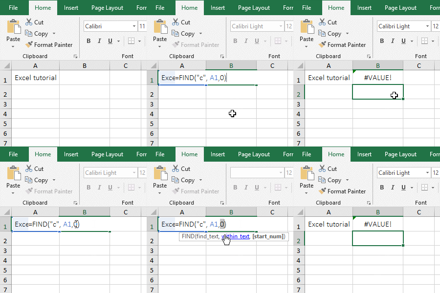
Figure 4

2. Formula description:

A. The formula =FIND("c",A1,0) finds from index 0, but returns an error, indicating that the Find function's Start_Num starts from 1.

B. The formula =FIND("c",A1,14) has a search start position of 14, and the "Excel tutorial" in A1 has only 14 characters. The formula finds the 15th character from the 14th character, therefore return an error.

(V) Cannot find the Find_Text return error and processing method

1. Double-click the cell B1, copy the formula =FIND("b",A1,1) to B1, press Enter, return the value error #VALUE!; double-click B1 again, and change the formula to =IFERROR(FIND("b",A1,1),0), press Enter, return 0; the operation steps, as shown in Figure 5:

Figure 5

2. Formula description:

A. Formula =FIND("b",A1,1) finds "b" from the first character in the "Excel Tutorial", but not found, it returns an error.

B.IfError function is an error judgment function in the formula =IFERROR(FIND("b",A1,1),0), meaning: If FIND("b",A1,1) returns the correct index, then IfError returns this value, otherwise returns 0.

Third, How to use findB function in excel

(I) Find in a string consisting of numbers and letters

1. Double-click the cell B1, copy the formula =FINDB("0",A1,6) to B1, press Enter, return to 8; the operation steps are as shown in Figure 6:

Figure 6

2. 0 is the Find_Text, A1 is the Within_Text, and 6 is the Start_Num in the formula =FINDB("0",A1,6); the formula means: finds 0 from the 6th characters from the "Excel 2019" in A1, and the index of 0 that is returned is 8. From the return index, the FindB function like Find function, counts numbers and letters as one byte.

IV, The application examples of Excel Find function and FindB function

(I) Mid + Find function combination to intercept the string from any specified character

1. If you want to intercept the middle Clothes Name in "WS-560Pink long sleeve shirt12.9". Double-click the cell B1, copy the formula =MID(A1,FIND("Pink",A1),22) to B1, press Enter, and return to the "Pink long sleeve shirt"; the operation steps are as shown in Figure 7:

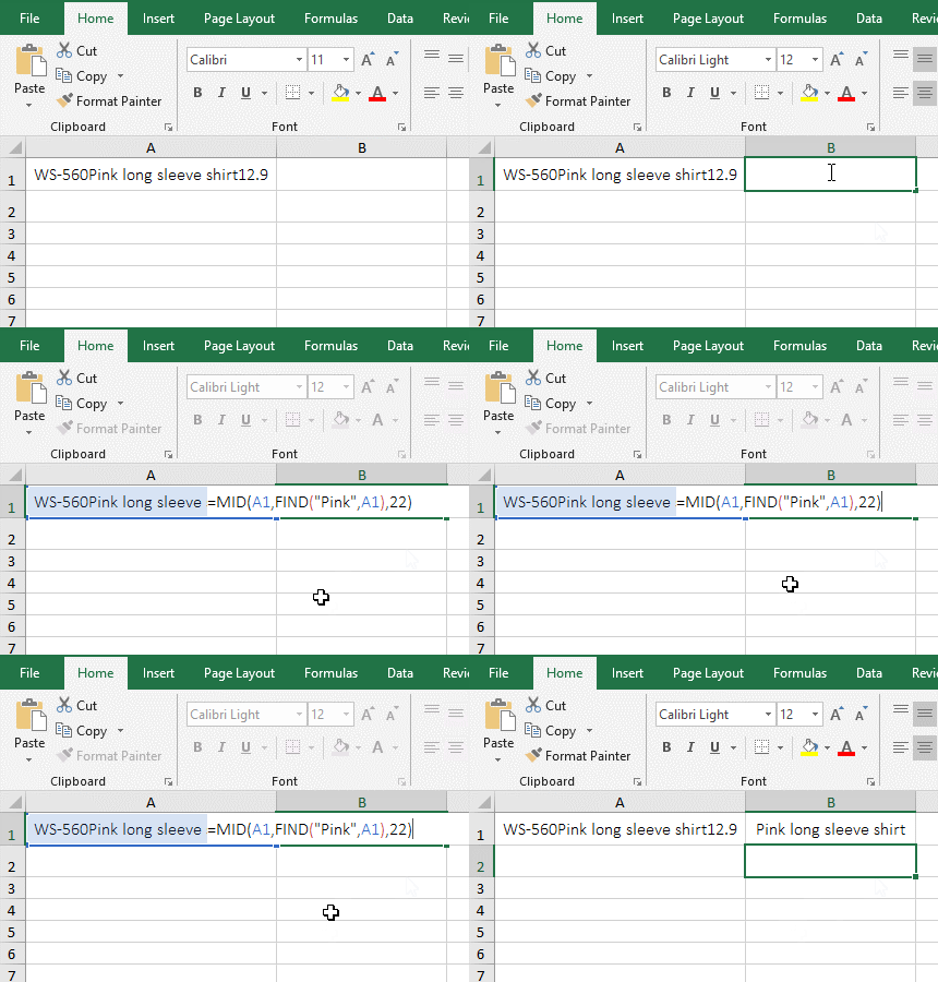
Figure 7

2. The formula =MID(A1,FIND("Pink",A1),22) description:

A. FIND("Pink",A1) is used to find the index of "Pink" in A1, the result is 7; when intercepting in a long string, usually use the Find function to determine the starting index of the string to be intercepted, so Can find quickly the starting index of the Find_Text, do not have to count one by one.

B. The formula becomes =MID(A1,7,22), A1 is the text to intercept the text, 7 is the starting interception index, and 22 is the intercept length, meaning: 22 characters are intercepted from the 7th character, just cut Get 22 characters in A1.

Hint: Mid + FindB or MidB + FindB can also achieve the same function, the formula can be written separately: =MID(A1,FINDB("Pink",A1),22) or =MIDB(A1,FINDB("Pink",A1),22).

(II) If + IsNumber + Find function combination to dynamic lookup

1. If it is required to indicate whether the column A contains the year of column B, if it is, marks "Yes", otherwise marks "No". Double-click the cell C2, copy the formula =IF(ISNUMBER(FIND(B2,A2)),"Yes","No") to C2, press Enter, return "Yes"; select C2 and move the mouse to the cell fill handle in the right lower corner of C2, after the mouse becomes the bold black plus, double-click the left button to mark the corresponding result of the remaining rows; the operation steps are as shown in Figure 8:

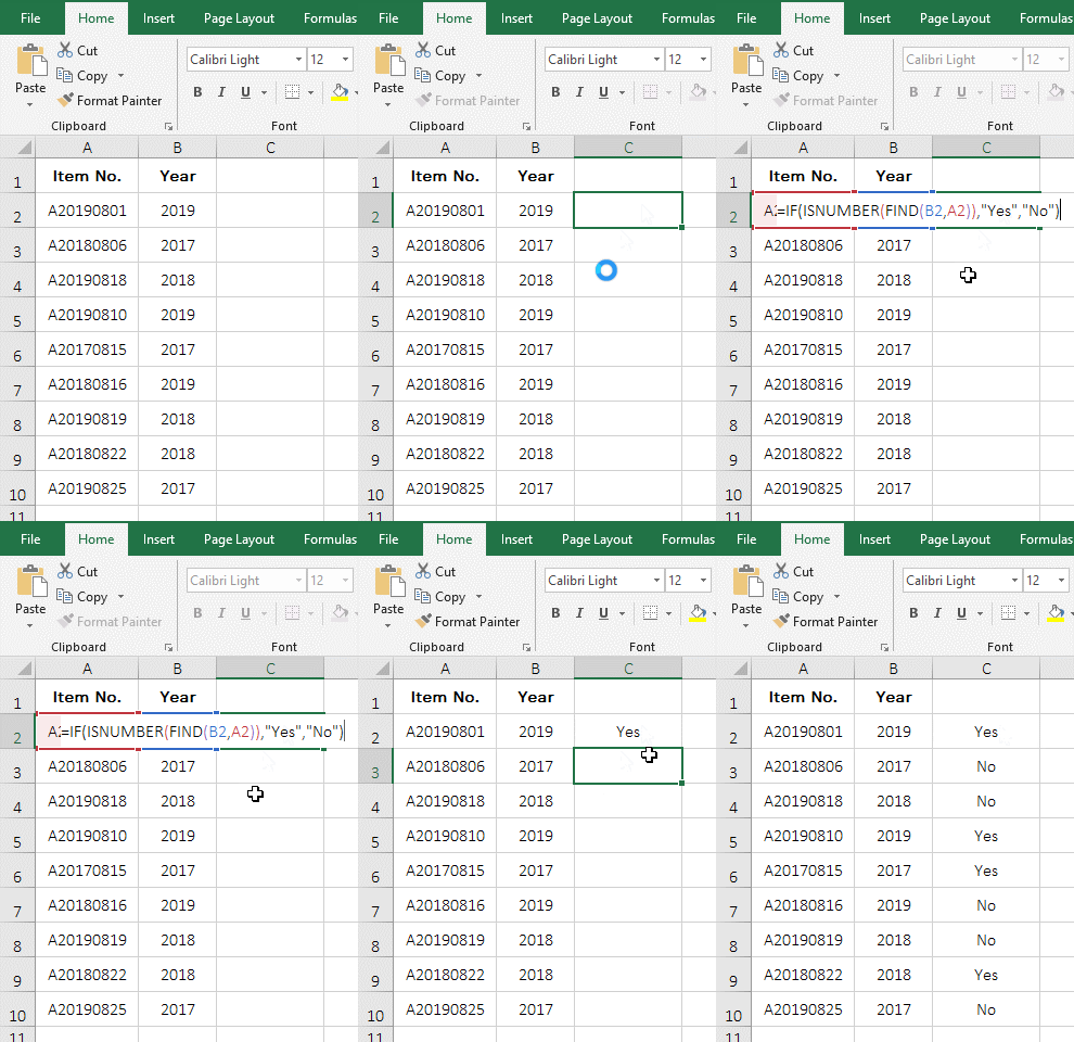
Figure 8

2. The formula =IF(ISNUMBER(FIND(B2,A2)),"Yes","No") description:

A. FIND(B2,A2) is used to find B2 in A2. If found, return the index of B2 in A2, otherwise the return the error value #VALUE!; when the formula is in C2, return the index of B2 in A2.

B. ISNUMBER(FIND(B2,A2) becomes ISNUMBER(2), since 2 is a number, so IsNumber returns "True". Then the formula becomes =IF(TRUE,"Yes","No"), the criteria of If is true, so return "Yes".

C. When the formula is in C3, both A2 and B2 automatically change to A3 and B3(equivalent to dragging down), FIND(B3,A3) returns the error value #VALUE!, because B3 is not found in A3; ISNUMBER(#VALUE!) returns "False", the formula becomes =IFFALSE,"Yes","No"), the criteria of If is false, so it returns "No".

(III) Sum + IsNumber + Find function combination to find multiple values at a time

1. If you want to find 4 values at a time. Double-click the cell B1, copy the formula =SUM(ISNUMBER(FIND({"S","shirt",9,10},A1))*1) to B1, press Enter, return to find result 3; operation steps as shown in Figure 9:

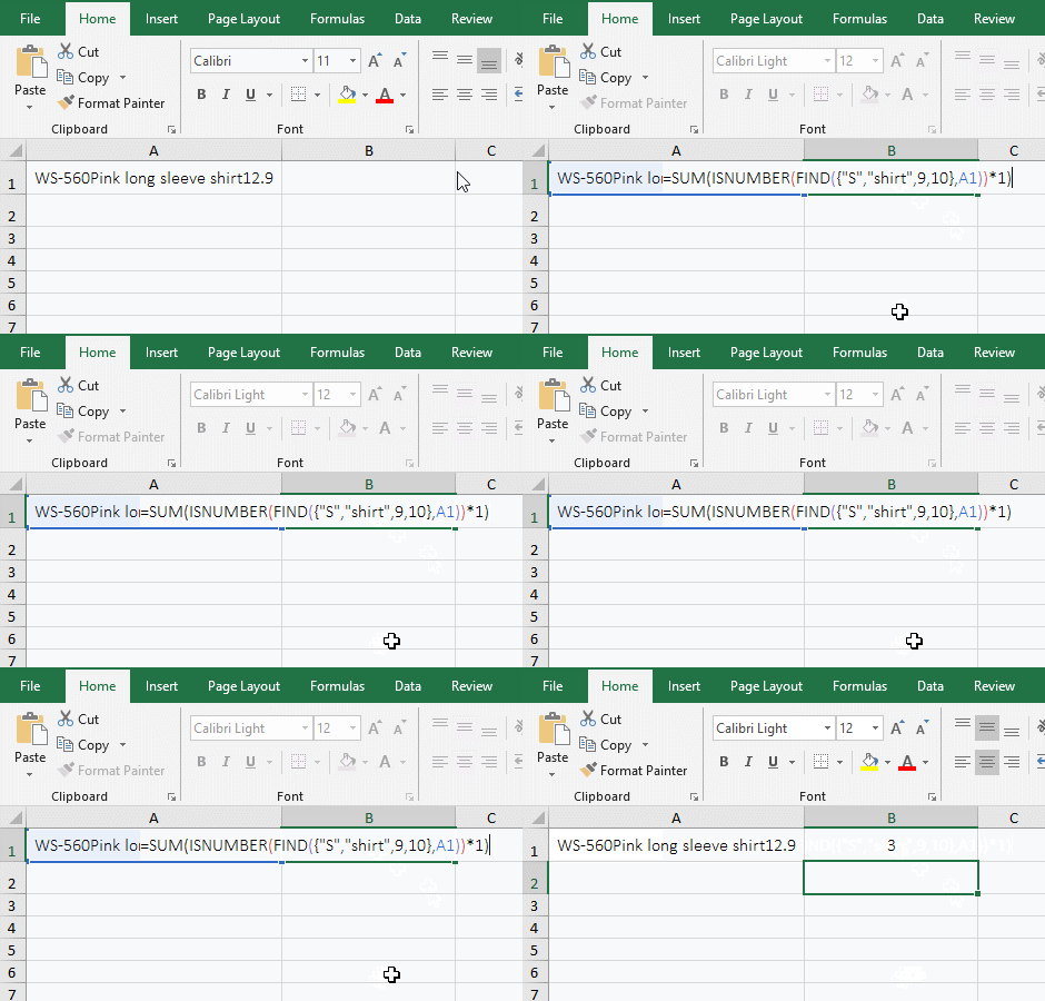
Figure 9

2. The formula =SUM(ISNUMBER(FIND({"S","shirt",9,10},A1))*1) description:

A. The Find_Text of FIND({"S","shirt",9,10},A1) is an array, the array contains 4 elements, that is, to find four values in A1; when executed, the first element S in the array is fetched for the first time, then it is looked up in A1, and the result is 2; the second element "shirt" in the array is fetched for the second time, it is also looked up in A1, and the result is 24; And so on, and finally return the array {2,24,32,#VALUE!}, since 10 is not found in A1, so #VALUE! is returned.

B. The formula becomes =SUM(ISNUMBER({2,24,32,#VALUE!})*1), and further calculates whether the element in the array is a number by IsNumber, and returns True if it is a number, otherwise returns False; the formula becomes =SUM({TRUE,TRUE,TRUE,FALSE}*1), and each element in the array is multiplied by 1(When multiplied, True turns to 1, and False turns to 0); the formula becomes =SUM({1,1,1,0}), and finally adds each element in the array with Sum, result to 3.