Excel left function usage(8 examples, with Sum+Value+Left to add the digital band units)

The Left function is used to extract the specified number of characters from the first character from the left, and the LeftB function is used to extract the specified number of bytes from the text starting from the first character on the left in excel; The former extracts the number of characters, that is, counts the full-width and half-width as one character; the latter extracts the number of bytes, that is, counts the full angle as two bytes and half-width as one byte.

The Left function and the LeftB function are often combined with functions such as If, Len, LenB, Find, Sum, Value, and Match in practical applications. For example, Left + Len(or LeftB + LenB) combines to implement reciprocal extraction of characters, If + Find combines to return an eligible search, Left + Find combination automatically calculates the number of characters to extract, and Sum + Value + Left combination implements add the numbers with unit.

I, Excel Left function and LeftB function syntax

1. Left function expression: LEFT(Text,[Num_Chars])

2. LeftB function expression: LEFTB(Text,[Num_Bytes])

3. Description:

A. Left function counts full-width(such as Chinese characters, Japanese characters and Korean characters) and half-width characters(such as numbers and letters) as one character, and LeftB function counts full-width characters as two bytes and half-width characters as one byte.

B. Num_Chars is to extract the number of characters, it must be greater than or equal to 0, otherwise it will return the value error #VALUE!; If Num_Chars is greater than the length of text, all text will be returned; if Num_Chars is omitted, the default is 1.

C. Num_Bytes is the number of bytes of the character to be extracted, it must be greater than or equal to 0, otherwise it will return the value error #VALUE!; if Num_Bytes is greater than the length of text(the half-width character is more than the length of text, the full-width character is greater than double the length of text), it will return all text; if Num_Bytes is omitted, it defaults to 1.

II, The examples of Excel Left function

(I) Extract the number instance on the left

1. If you want to extract the number to the left of the unit. Select the cell B1, enter the formula =LEFT(A1,3), press Enter, return to 2.5; select B1, move the mouse to the cell fill handle in the lower right corner of B1, and after the mouse becomes the bold balck plus, double-click the left button, then return the number before the remaining units; the operation process steps, as shown in Figure 1:

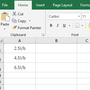
Figure 1

2. A1 is the Text to extract the number, 3 is the Num_Chars in the formula =LEFT(A1,3); the formula means that the "2.5 liter/bottle" in A1 is extracted from the first character and only Extract 3 characters.

(II) Extract a character or all text

1. Select the cell A8, enter the formula =LEFT(A5,), press Enter, return to "empty"; double-click A8, remove the comma, press Enter, return to "G"; double-click A8 again, enter after A5 ", 6", press Enter to return to "Grape"; the operation steps are as shown in Figure 2:

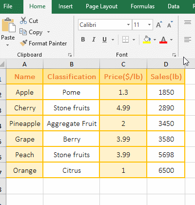
Figure 2

2. Formula description:

A. Formula =LEFT(A5,) returns null, and the formula =LEFT(A5) returns "G", indicates that when the argument Num_Chars is omitted, there can be no comma; in addition, when  Num_Chars is omitted, its value defaults is 1.

B. Formula =LEFT(A5,6) returns 6 characters from the first character. Since there are only 5 characters in A5, only the end of the text is returned, that is, all characters are returned.

(III) The number of extracted characters is less than 0, return #VALUE! Error

1. Double-click the cell B1, copy the formula =LEFT(A1,-1) to B1, press Enter, return the value error #VALUE!; double-click B1, change -1 to 1, press enter, return 2; double-click B1 again, change 1 to 0, press Enter, return to "empty"; the operation steps, as shown in Figure 3:

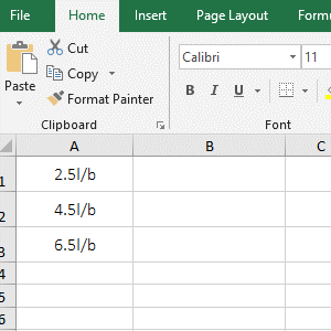
Figure 3

2. Formula =LEFT(A1,-1) returns an error because the second argument Num_Chars must be greater than or equal to 0; formula =LEFT(A1,1) returns the first character 2 in A1; formula =LEFT(A1,0) returns "Empty" because the Num_Chars is 0.

III, The examples of Excel LeftB function

(I) Extract numbers and letters

1. If you want to extract weight and unit from column A. Select the cell B1, enter the formula =LEFTB(A1,3), press Enter, return 3kg; move the mouse to the cell fill handle in the lower right corner of B1, and then double-click to extract the weight and unit of the remaining cells; operation process steps, as shown in Figure 4:

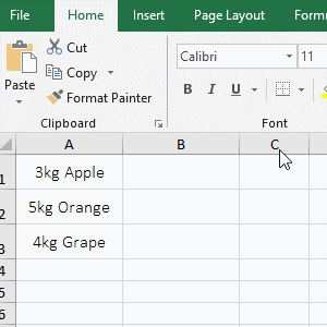
Figure 4

2. A1 is the Text to extract the character, 3 is the Num_Bytes in formula =LEFTB(A1,4); the formula means that extracts 3 bytes from the first character from "3kg Apple" in A1, ie extracts "3kg"; from the returned results, the LeftB function, like the Left function, counts numbers and letters as one byte.

IV, The application example of Excel Left function and LeftB function

(I) Left + Len function combination to achieve reciprocal extraction of characters

1. If you want to extract from the 8th last digit. Double-click the cell B2, copy the formula =LEFT(A2,LEN(A2)-8 + 1) to B2, press Enter, return to 2019; the operation steps are as shown in Figure 5:

Figure 5

2. Formula =LEFT(A2,LEN(A2)-8 + 1) explanation:

A. The 8 in the formula is the starting position of the reciprocal extraction, that is, the 8th character from the right to the left is extracted; LEN(A2) is used to return the number of characters of the text in A2, and the result is 11. The Len function takes the full-width character or the half-width Characters are counted as one character.

B. The formula becomes =LEFT(A2,11 - 8 + 1), and the further calculation becomes =LEFT(A2,4), that is, extracts from the left side, 4 characters are extracted, and the result is 2019.

Tip: LeftB + LenB can also achieve the same function, the formula can be written like this: =LEFTB(A2,LENB(A2)-8 + 1), copy the formula to B3, press enter, also return to 2018, the operation steps, such as Figure 6 shows:

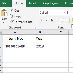
Figure 6

8 is also the position where the reciprocal extraction character starts in the formula =LEFTB(A2,LENB(A2)-8 + 1), and LENB(A2) returns the number of bytes of text in A2, the result is 11, and the LenB function counts the full-width character as 2 bytes and half-width characters are counted as 1 byte, which is the same as LeftB; the formula becomes =LEFTB(A2,4), and then 4 bytes of characters are extracted from the left.

(II) If + Left function combination to return the values that meet special criteria

1. If you want to find out the "Position" of all employees with starting "S". Double-click the cell D2, copy the formula =IF(LEFT(A2)="S",C2,"") to D2, press Enter to return the null value; select D2, and with the double-click the cell fill handle to find the "Position" of the remaining employee; the operational process steps, as shown in Figure 7:

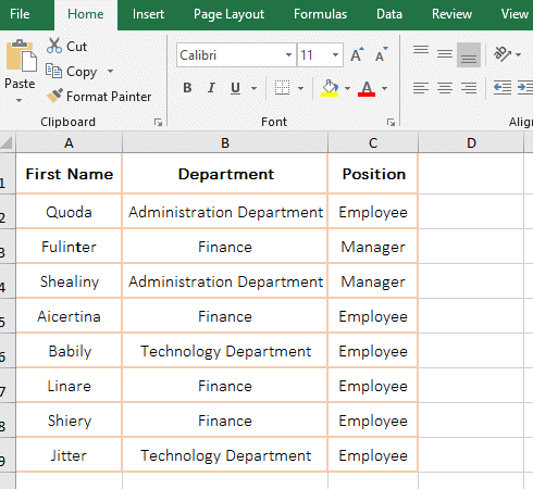
Figure 7

2. Formula =IF(LEFT(A2)="S",C2,"") description:

A. LEFT(A2) is used to intercept the letter "S" in the "First Name" in A2; LEFT(A2)="S" is the condition of If, if the result returned by LEFT(A2) is equal to "S", then return C2, otherwise return empty value.

B. When the formula is in D2, LEFT(A2) returns "Q", which is not equal to "S", so it returns a null value; when the formula is in D4, A2 automatically changes to A5, LEFT(A4), returns "S", so return C4(the "Manager").

(III) Left + Find function combination to calculation automatic to extract the number of characters

1. when you want to extract characters from long text or only extract specific characters, you can use the Find function to return the position of a character, and then use the Left function to extract. Suppose you want to extract the string from the start character to 5 in A2. Double-click the cell B2, copy the formula =LEFT(A2,FIND(5,A2)) to B2, press Enter, return to A201909010005; the operation steps are as shown in Figure 8:

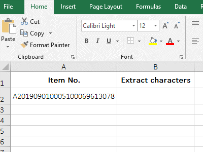
Figure 8

2. Formula =LEFT(A2,FIND(5,A2)) explanation:

A. FIND(5,A2) is used to return the position of 5 in A2 (the result returns 13), 5 is to find the text, the text in A2 is to find the original text of 5, FIND(5,A2) omits the last argument that specifies the search start position, by default, starts from the first character.

B. The formula becomes =LEFT(A2,13), and finally 13 characters are intercepted from the first character on the left, that is, A201909010005 is obtained.

(IV) Sum + Value + Left function combination to add the digital band units

1. If the numbers are followed by a unit, they cannot be added with the Sum function. The Numbers need to be extracted first and then summed. If you want a sum of sales of a fruit table. Double-click the cell D8, copy the formula =SUM(VALUE(LEFT(D2:D7,4))) to D8, press Ctrl + Shift + Enter to return to the summation result 23968; the operation steps are as shown in Figure 9:

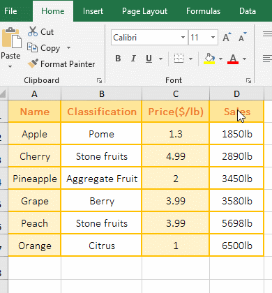
Figure 9

2. The formula =SUM(VALUE(LEFT(D2:D7,4))) description:

A, The formula is an array formula, so press Ctrl + Shift + Enter. D2:D7 returns the values in D2 to D7 as an array, ie {"1850lb";"2890lb";"3450lb";"3580lb";"5698lb";"6500lb"}.

B. Then LEFT(D2:D7,4) becomes LEFT({"1850lb";"2890lb";"3450lb";"3580lb";"5698lb";"6500lb"},4), when executed, the first element "1850lb" in the array is taken out for the first time, and the first four digits are truncated, that is, 1850; the second element in the array is taken out for the second time, and the first four digits are also intercepted, that is, 2890; analogy, and finally returns {"1850";"2890";"3450";"3580";"5698";"6500"}.

C. The formula becomes =SUM(VALUE({"1850";"2890";"3450";"3580";"5698";"6500"})), further calculation, use the Value function to convert the character elements in the array When to a value, the formula becomes =SUM({1850;2890;3450;3580;5698;6500}), and finally summed with the Sum function.