Excel Search function and SearchB usage(13 examples,include find multiple values and with Mid,Index)

The Search function is used to find the position of the specified text in the text of the search text in Excel. The SearchB function has the same function as the Search function, but they differ, the Search function takes a full-width(such as Chinese characters, Japanese characters and Korean characters) and a half-width(such as numbers and letter) are counted as one character, and the SearchB function counts full-width characters as two bytes and half-width characters as one byte when you have enabled the editing of a language that supports DBCS and then set it as the default language. In addition, the difference between the Search and SearchB function and the Find and FindB function is that the first two are case-insensitive and fuzzy lookup with wildcard is allowed, the latter two are case-sensitive and wildcards are not allowed.

The Search and SearchB function can be combined with functions such as Mid, Sum, Index, Match, IsNumber, and Count. For example, the combination of Mid + Search (or SearchB) implements interception of the specified string, and the combination of Count + Search function counts the number of cells that contain the specified text in the column, the combination of Sum + IsNumber + Search function can find multiple values at a time, and the Index + Match + IsNumber + Search function combination returns the corresponding cells that match in the two columns.

I, Excel Search function and SearchB function syntax

1. Search function expression: SEARCH (Find_Text, Within_Text, [Start_Num])

2. SearchB function expression: SEARCHB (Find_Text, Within_Text, [Start_Num])

3. Description:

A. Search function counts each character as a byte, whether it is a half-width character(such as "number or letter") or a full-width character(such as Chinese characters, Japanese characters and Korean characters); SearchB function counts half-width characters as 1 byte, full-width characters as 2 bytes. Both the Search and SearchB function ignore case-insensitive, and can also use a wildcard question mark(?) or an asterisk(*); the Find and FindB function require case sensitivity and cannot use wildcards, which is also their difference.

B. You can use the wildcard question mark(?) or asterisk(*) in Find_Text. The question mark means any character. The asterisk indicates any one or more characters. If you want to find wildcards, you need to add the escape character ~ in front of them. Then find the question mark as ~?, and find the asterisk as ~*.

C. If you find empty text(""), return the position 1 of the first character.

D. Start_Num is optional, if omitted, it starts from the first character; if Start_Num is less than or equal to 0 or greater than or equal to the length of Within_Text, Search and SearchB both return the value error #VALUE!.

E. If the Find_Text is not found in Within_Text, the value error #VALUE! is also returned.

II, The examples of Excel Search function

(I) Find a word or phrase

1. Select the cell B1, copy the formula = SEARCH("tutolail", A1) to B1, press Enter, return to 16; select B2, enter the formula =SEARCH("return to",A2), press Enter, return to 17; the operation steps are as shown in Figure 1:

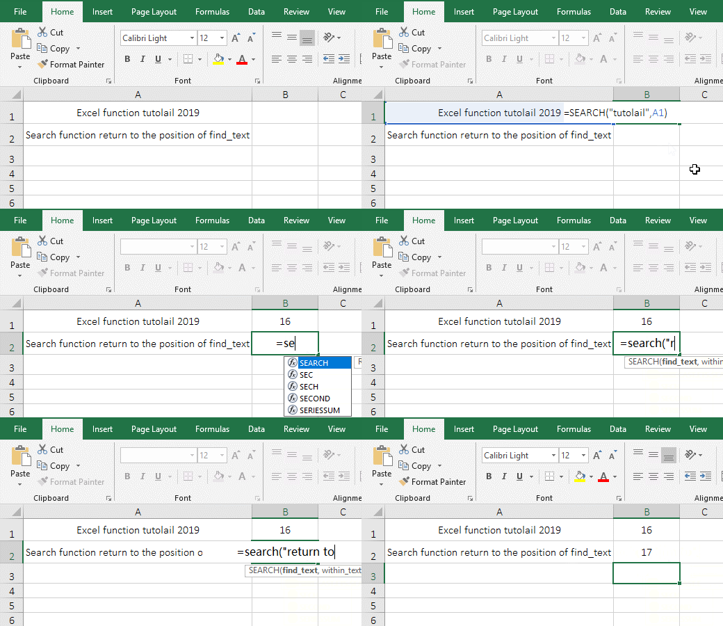
Figure 1

2. Formula description:

A. The word "tutolail" is the Find_Text, A1 is the Within_Text in the formula =SEARCH("tutolail",A1), the formula means: find the tutolail in A1 and return the position of the first letter t of tutolail in A1.

B. Formula =SEARCH("return to",A2) means: look up "return to" in A2 and return to the position of the first word "return" in A2.

(II) Examples of using wildcards ? and *

(1) Use *

1. If you want to find the "option" in the "Excel function option tutolail". Double-click the cell B1, copy the formula =SEARCH("o*n",A1) to B1, press Enter, return to 13; double-click B1, change "o*n" to "op*n", press Enter, return to 16; the operation steps are as shown in Figure 2:

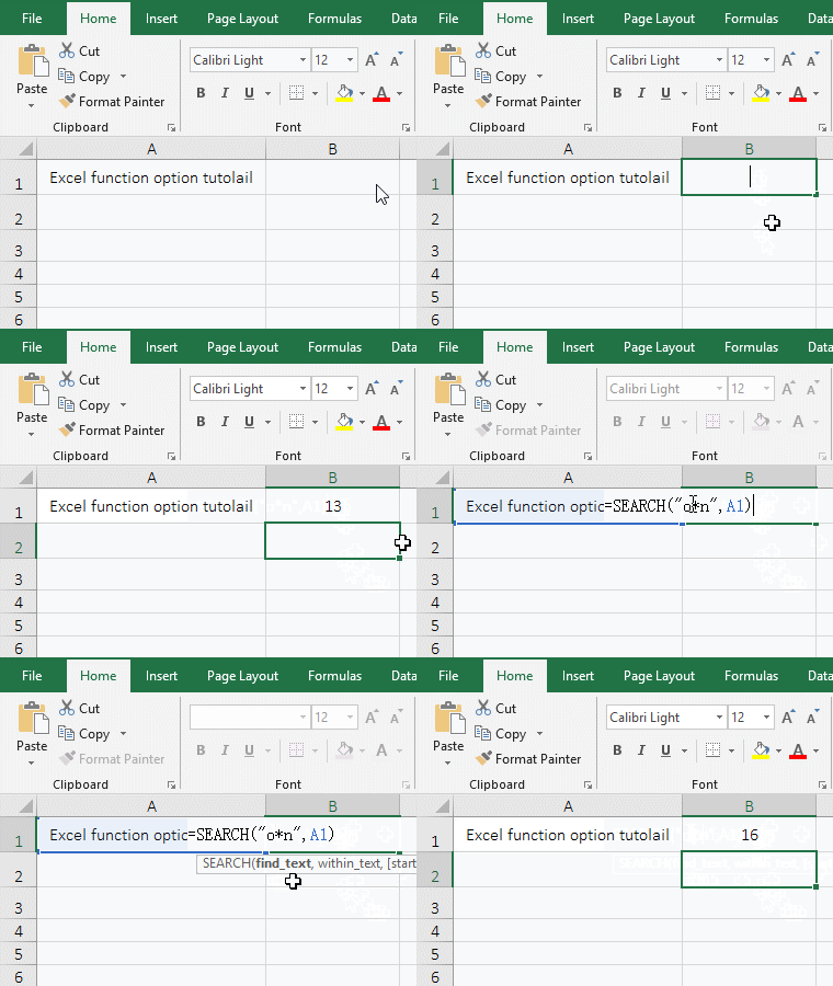
Figure 2

2. Formula description:

The Find_Text "n*o" in the formula =SEARCH("o*n",A1) has an asterisk, which means to find a string starting with "n" and ending with "o", and at least three eligible in "Excel function option tutolail", ie "on, option", and "on option", and return 13 is the location of "on", so to find the "option", you must add "p" after the "o" of "o*n".

(2) use?

1. Also look for the "option" in the "Excel function option tutolail". Double-click the cell B1, copy the formula =SEARCH("o????n",A1) to B1, press Enter, return to 16; the operation steps are as shown in Figure 3:

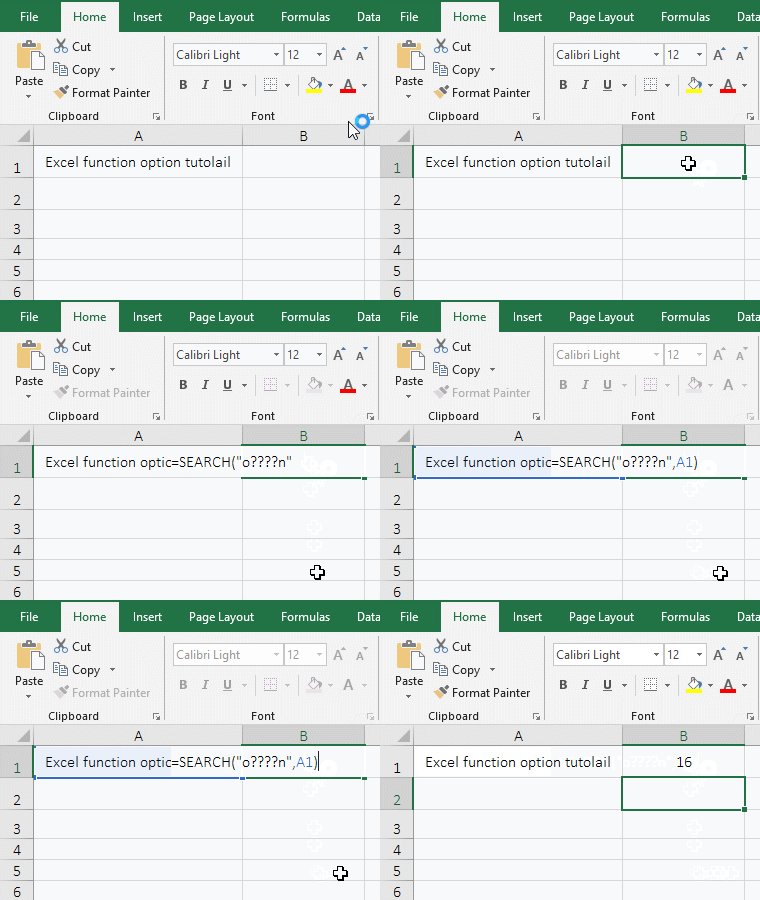
Figure 3

2. Formula description:

The Find_Text o????n in the formula =SEARCH("o????n",A1) has four question marks, each question mark represents a character, meaning that finds the string that starts with "n" and ends with "o" and there is only four characters between "n" and "o", so just return the position of the word "option" in A1.

(III) Find empty text("") and spaces(" ")

1. Double-click the cell B1, copy the formula =SEARCH("",A1) to B1, press Enter, return to 1; double-click B1 again, position the mouse in double quotes "", press the space on the keyboard, add a space in the double quotes, press Enter, return to 6; the operation steps, as shown in Figure 4:

Figure 4

2. Formula =SEARCH("",A1) find empty text(""), the Search function returns the position 1 of the first character by default; formula =Search(" ",A1) find spaces, return position 6 of the first space in "Excel function option tutolail".

(IV) Find double quotation marks(")

1. Double-click the cell B1, copy the formula =SEARCH("""",A1) to B1, press Enter, return to 7; the process steps, as shown in Figure 5:

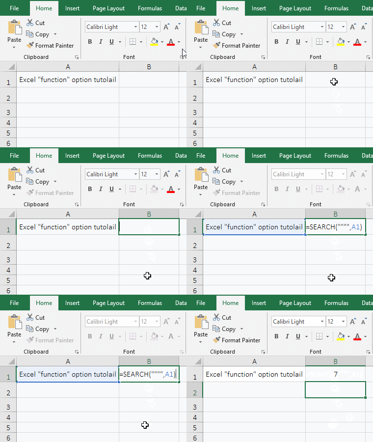
Figure 5

2. Formula description:

The formula =SEARCH("""",A1) Find the double quotes ", it is worth noting that you must enter two double quotes, so the returned position is still the position of the first double quote.

(V) Start_Num is not in scope and causing #VALUE!

1. Double-click the cell B1, copy the formula =SEARCH("function",A1,0) to B1, press Enter, return the value error #VALUE!; double-click B1, change 0 to 1, press Enter, return 7 Double-click B1 again, change 1 to 30, press Enter, return #VALUE!; operation steps, as shown in Figure 6:

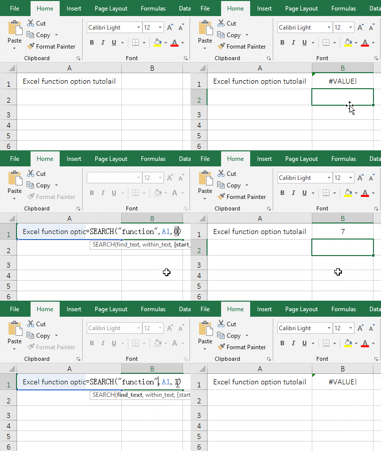
Figure 6

2. Formula description:

A. 0 means to start from the 0th character in formula =SEARCH("function",A1,0), but the Search function requires at least the first character to start looking, so return an error; change 0 to 1, immediately returns the "function" in the correct position in A1.

B. Formula =SEARCH("function",A1,30) searchs from the 30th character, but the starting position of "function" is 7, so an error is returned.

(VI) Cannot find text return error and processing method

1. Double-click the cell B1, copy the formula =SEARCH("3",A1) to B1, press Enter, return the value error #VALUE!; double-click B1 again, and change the formula to =IFERROR(SEARCH("3",A1),"NO FOUND"), press Enter, return "Not Found"; the operation steps are as shown in Figure 7:

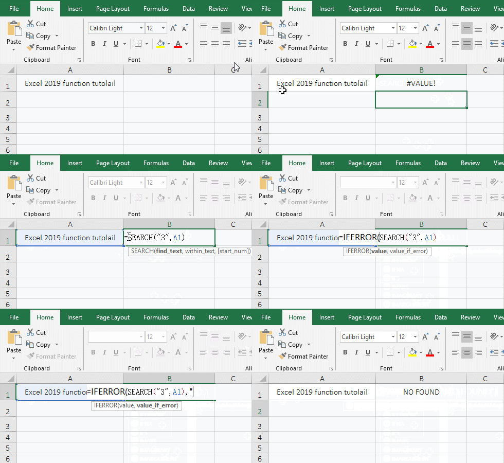
Figure 7

2. Formula description:

A. Formula =SEARCH("3",A1) finds 3 in the "Excel 2019 function tutolail", but not found, so returns value error.

B. The IfError function is used for processing When an error occurs when the formula SEARCH("3",A1) is executing in the formula =IFERROR(SEARCH("3",A1),"NO FOUND"), if SEARCH("3",A1) returns an error, IfError returns "not found", otherwise it returns the return value of SEARCH("3",A1).

III, The examples of Excel SearchB function

(I) An example of using a wildcard asterisk *

1. Double-click the cell B1, copy the formula =SEARCHB("o*n",A1) to B1, press Enter, return to 13; double-click B1 again, enter ",14" after A1, press Enter, return to 16 ; operation process steps, as shown in Figure 8:

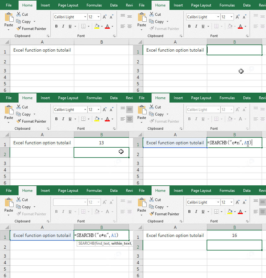
Figure 8

2. Formula description:

A. Find_Text "o*n" uses * in formula =SEARCHB("o*n",A1), which means to find a string starting with o and ending with n, the return value is 13, which is the position of "on" in A1.

B. The formula =SEARCHB("o*n",A1,14) is also looking for "o*n", but starting from the 14th character, so returning the position 16 of the word "option".

(II) An example of using a wildcard question mark ?

1. Double-click the B1 cell, copy the formula =SEARCHB("o????n",A1) to B1, press Enter, return to 16; process steps, as shown in Figure 9:

Figure 9

2. Formula description:

The Find_Text "o????n" of formula =SEARCHB("o????n", A1) uses four question marks?, each question mark represents a character, meaning: look up a string that begins with "o" and ends with "n" and only four characters between "o" and "n".

IV, Excel Search function and SearchB function application examples

(I) Mid + Search function combination to intercept the specified string

1. If you want to extract the "Excel 2019 Function Basic Tutorial" from the "Excel function Excel 2019 function basic tutorial option tutolail". Double-click the cell A2, copy the formula =MID(A1,SEARCH("e*l",A1,5),SEARCH("tutorial",A1)+LEN("tutorial")-SEARCH("e*l",A1,5)+1) to A2, press Enter, return to "Excel 2019 Function Basic Tutorial"; the operation process steps, as shown in Figure 10:

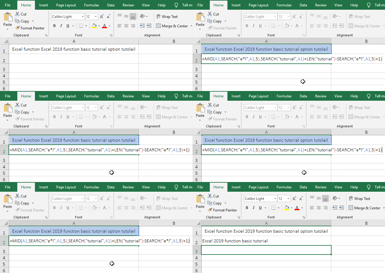
Figure 10

2. Formula =MID(A1,SEARCH("e*l",A1,5),SEARCH("tutorial",A1)+LEN("tutorial")-SEARCH("e*l",A1,5)+1) explanation:

A. SEARCH("e*l",A1,5) is used to search for the word starting with "e" and ending with "l" starting from the 5th character in A1, that is, intercepting the beginning word of the string to be searched for "Excel", because there is already an Excel before, so start with the 5th character to skip the first Excel; SEARCH("e*l",A1,5) has a return value of 16.

B. SEARCH("tutorial",A1) is used to return the position of the last word "tutorial" of the string to be intercepted in A1, the result is 42; LEN("tutorial") is used to count the number of characters of "tutorial"; SEARCH("tutorial",A1)+LEN("tutorial")-SEARCH("e*l",A1,5)+1) is used to calculate the length of the string to be truncated. The substitution value is 42 + 8 - 16 + 1 = 35. If only 50 - 16, the number of the truncated string will be one less, so 1 is added.

C. The formula becomes =MID(A1,16, 35), and finally 17 characters are intercepted from the 35th character in A1, which is the "Excel 2019 Function Basic Tutorial".

Tip: MidB + SearchB can also achieve the same function, the formula can be written like: =MIDB(A1,SEARCHB("e*l",A1,5),SEARCHB("tutorial",A1)-SEARCHB("e*l",A1,5)+LENB("tutorial")).

(II) Count + Search function combination to count the number of cells containing the specified text in the column

1. If you want to count the number of cells that contain the specified characters in the A column. Double-click the cell A11, copy the formula =COUNT(SEARCH("*"&C3&"*",A$2:A$8)) to A9, press Ctrl + Shift + Enter, return to 3; the operation steps are as shown in Figure 11:

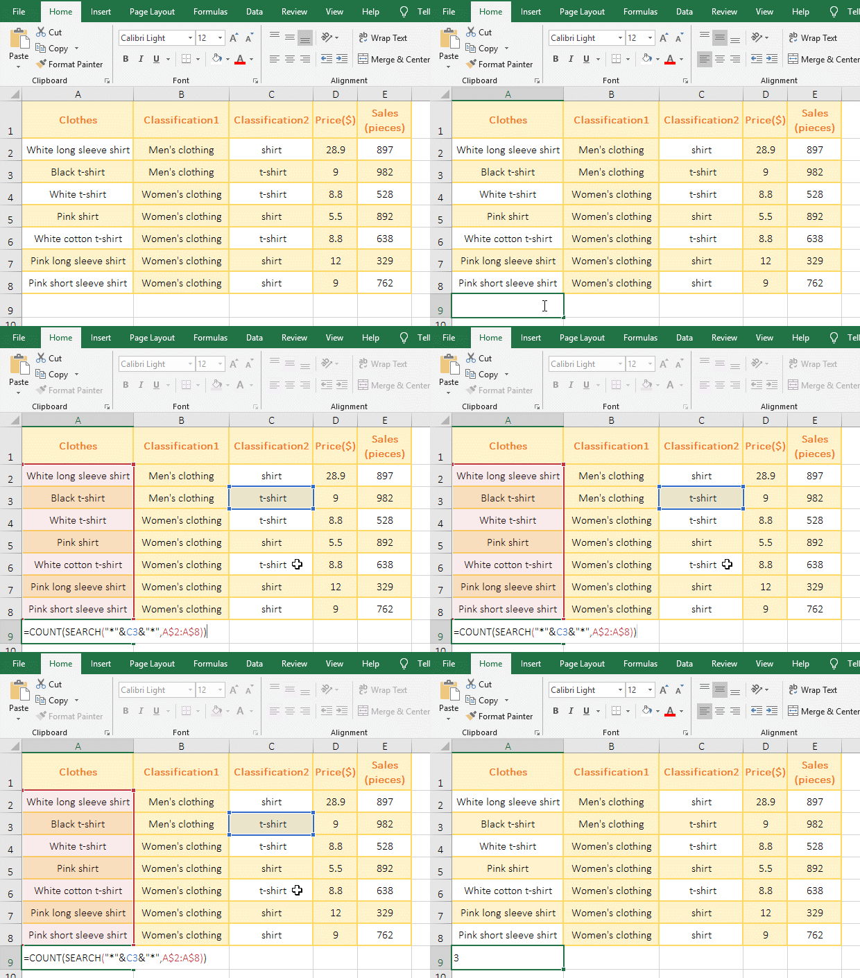
Figure 11

2. Formula =COUNT(SEARCH("*"&C3&"*",A$2:A$8)) description:

A. "*"&C3&"*" means to find text with C3 in the middle and any characters on both sides, and * can also be empty text(ie "").

B. A$2 is an relative reference to the column and absolute reference to the row, the $ before 2 means the absolute reference, that is, when dragging down, A2 will not change to A3, A4, etc.; A$2:A$8 returns All values in A2:A10 as an array.

C. When SEARCH("*"&C3&"*",A$2:A$8) is executed, "*"&C3&"*" becomes "*shirt*"; then, A2 is taken out from A2 to A8 for the first time, then Look for "*shirt*" in A2, return 1 because it is found; take A3 for the second time, "* shirt*" is not found, so the return value is wrong #VALUE!; the others and so on, and finally return the array {#VALUE!;1;1;#VALUE!;1;#VALUE!;#VALUE!}.

D. The formula becomes =COUNT({#VALUE!;1;1;#VALUE!;1;#VALUE!;#VALUE!}), and finally counts the number of elements in the array, due to #VALUE! No statistics, so the result is 3.

(III) Sum + IsNumber + Search function combination to find multiple values at a time

1. If you want to find 4 values at the same time. Double-click the cell A2, copy the formula =SUM(ISNUMBER(SEARCH({"excel","function",2016,2019},A1))*1) to A2, press Enter, return to the search result 3; As shown in Figure 12:

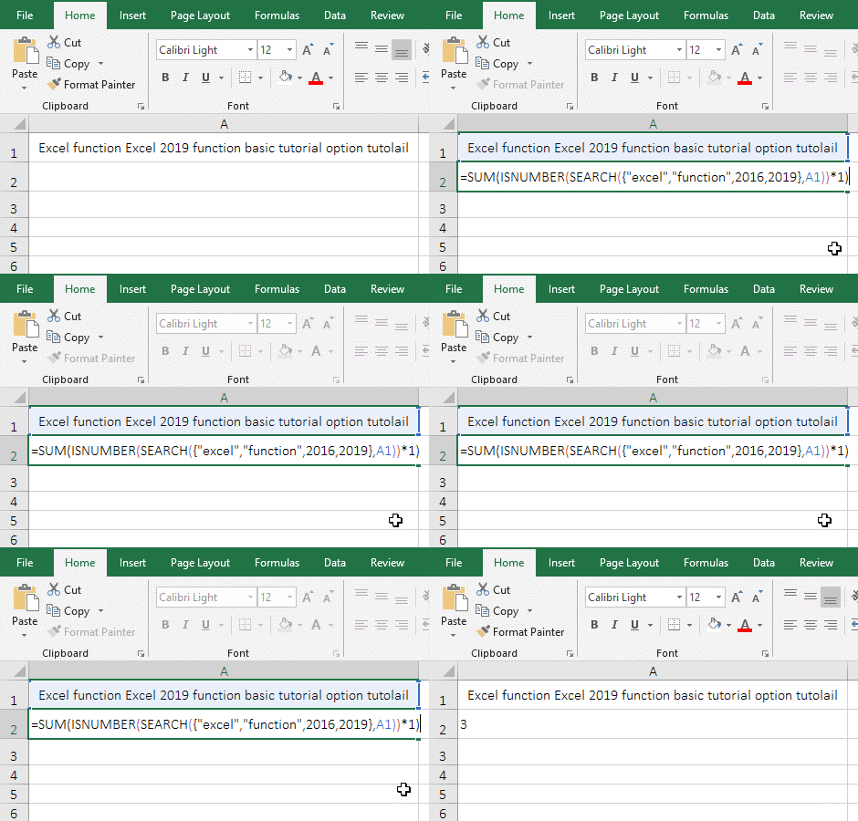
Figure 12

2. The formula =SUM(ISNUMBER(SEARCH({"excel","function",2016,2019},A1))*1) description:

A. The Find_Text of SEARCH({"excel","function",2016,2019},A1) is an array of 4 elements, that is, to find 4 values in A1; when executed, the first element "excel" is taken from the array for the first time, then it is searched in A1, and the result is 1; the second element "function" is taken from the array for the second time, and it is also searched in A1, the result is 7; the others and so on, and finally returns {1,7,#VALUE!,22}, because 2016 is not found in A1, so #VALUE! is returned.

B. The formula becomes =SUM(ISNUMBER({1,7,#VALUE!,22})*1), then, use IsNumber to check whether the elements in the array are numbers, if yes, return True, otherwise return False; Then the formula becomes =SUM({TRUE,TRUE,FALSE,TRUE}*1), and further calculates that each element in the array is multiplied by 1, when multiplied, True turns to 1, and False turns to 0, then the formula becomes =SUM({1,1,0,1}), and finally adds each element in the array, result is 3.

(IV) Index + Match + IsNumber + Search function combination returns the corresponding cells of the two columns matching

1. If the "Item No." in column A contains "column" in column B, the corresponding "quantity" is returned. Double-click the cell D2, copy the formula =INDEX(C$2:C$8,MATCH(1=1,ISNUMBER(SEARCH(B$2:B$8,A2)),)) to D2, press Ctrl + Shift + Enter, return to 870; move the mouse to the cell fill handle in the lower right corner of D2, after the mouse becomes the bold black plus, hold down the left button and drag down to return the remaining "quantity"; the operation steps are as shown in Figure 13:

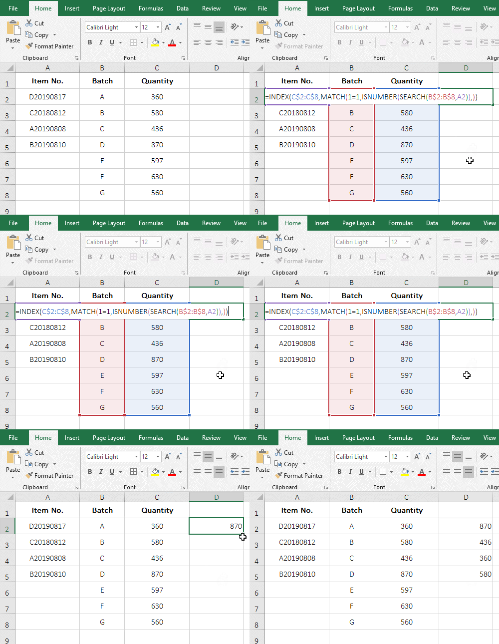
Figure 13

2. Formula =INDEX(C$2:C$8,MATCH(1=1,ISNUMBER(SEARCH(B$2:B$8,A2)),)) description:

A. B$2:B$8 returns the values in B2 to B8 as an array, ie {"A";"B";"C";"D";"E";"F";"G"}; SEARCH(B$2:B$8,A2) becomes SEARCH({"A";"B";"C";"D";"E";"F";"G"},A2), then take each element out of the array and look it up in A2, returns 1 if found, otherwise returns #VALUE!; finally returns {#VALUE!;#VALUE!;#VALUE!;1;#VALUE!;#VALUE!;#VALUE!}.

B. ISNUMBER(SEARCH(B$2:B$8,A2)) becomes ISNUMBER({#VALUE!;#VALUE!;#VALUE!;1;#VALUE!;#VALUE!;#VALUE!}), further calculate, use IsNumber to determine each element of the array, if it is a number, return True, otherwise return False; finally return {FALSE;FALSE;FALSE;TRUE;FALSE;FALSE;FALSE}.

C. 1=1 is used to return True, because the array elements returned by IsNumber are True and False, which is easy to judge.

D. Then MATCH(1=1,ISNUMBER(SEARCH(B$2:B$8,A2)),) becomes MATCH(TRUE,{FALSE;FALSE;FALSE;TRUE;FALSE;FALSE;FALSE},), then, Look for True in the array, return to its position in the array, and finally return 4.

E. The formula becomes =INDEX(C$2:C$8,4), and finally the value of the fourth row from C2 to C8 is returned by the Index function, which returns 870.