How to round numbers in excel and fix rounding errors(13 examples, with amount difference 0.1)

If you want to round a number to the specified decimal place, you can use the numeric function and the Round function in Excel. There are three ways for the number function; one is to use the "decrease decimal places", the second is to use the "number format", and the third is to use the "numeric value". The first and third ways can choose the number of digits to be rounded. The second way rounds only two decimal places; however, the integers are rounded with decimal places in the three ways above. The numbers are not only rounded to any number of decimal places, but the integers do not retain decimals with the Round function, especially when integers are not allowed to retain decimals. In addition, the Round function can be used to achieve when the number behind the numbers to be rounded the number of decimal places is greater than or equal to 3, carries 1 to the number before it.

If you want to automatically round, you can first set the number of decimal places to be rounded in the cell, and the value to be  inputted will be automatically rounded. If you only want to keep the decimals and do not round off, you can use the Trunc function and RoundDown function. If you want to round to a specified multiple, you can use the MRound function. The following are 13 examples of Excel round, not only including the issues above, but also the sum of amounts are difference 0.1, the sum of percentage is not equal to 100%, and the amount after the salaries are rounded  is more or less than a few cents.

I, Method 1 of how to round numbers in excel: Use "Number" function

1. Round to two decimal places with the "Decrease Decimal"

Select the cell that you want to round to two decimal places(such as A2:A4), the current tab is "Home", click the "Decrease Decimal" icon in the "Number" group, the selected values will be reduced by one decimal place and rounded; operation process steps, as shown in Figure 1:

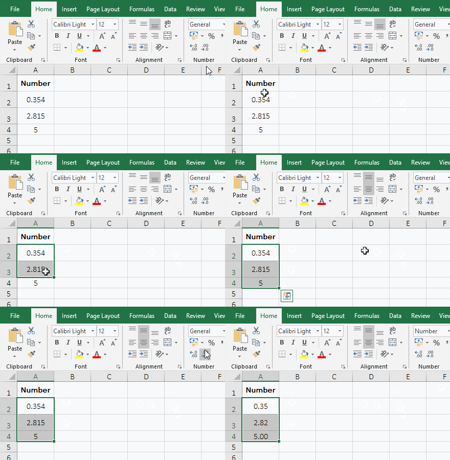
Figure 1

2. Round to two decimal places with the "Number Format"

Select the two cells A2:A4, the current is the "Home" tab, click the drop-down list box of the "Number Format"(There is the "General" in it) above the "Number", and select the "Number" in the pop-up options", Then the numbers of A2:A4 are rounded to two decimal places; the operation steps are shown in Figure 2:

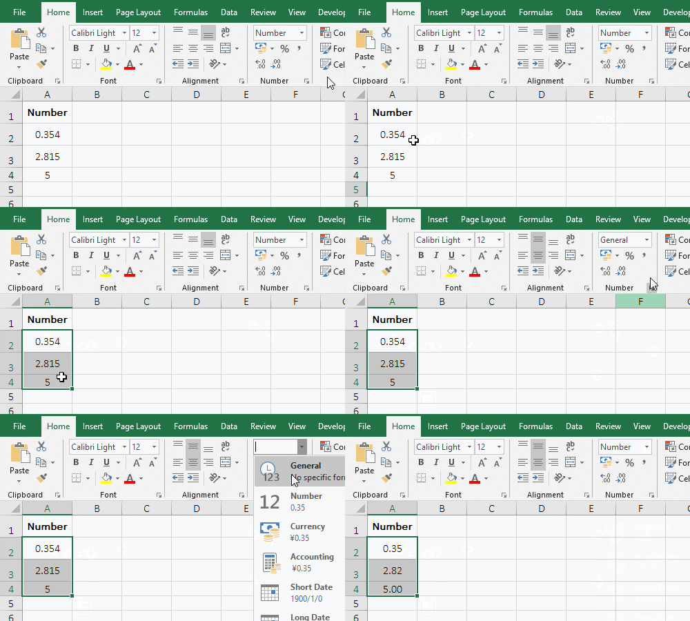
Figure 2

3. Round the value to two decimal places with the "Number"

Similarly, select the three cells A2:A4, press Ctrl + 1, open the "Format Cells" dialog box, select the "Number" tab, select "Number" on the left, the value of "Decimal places" is 2, click "OK", the number in the selected cells are rounded to two decimal places; the operation steps are shown in Figure 3:

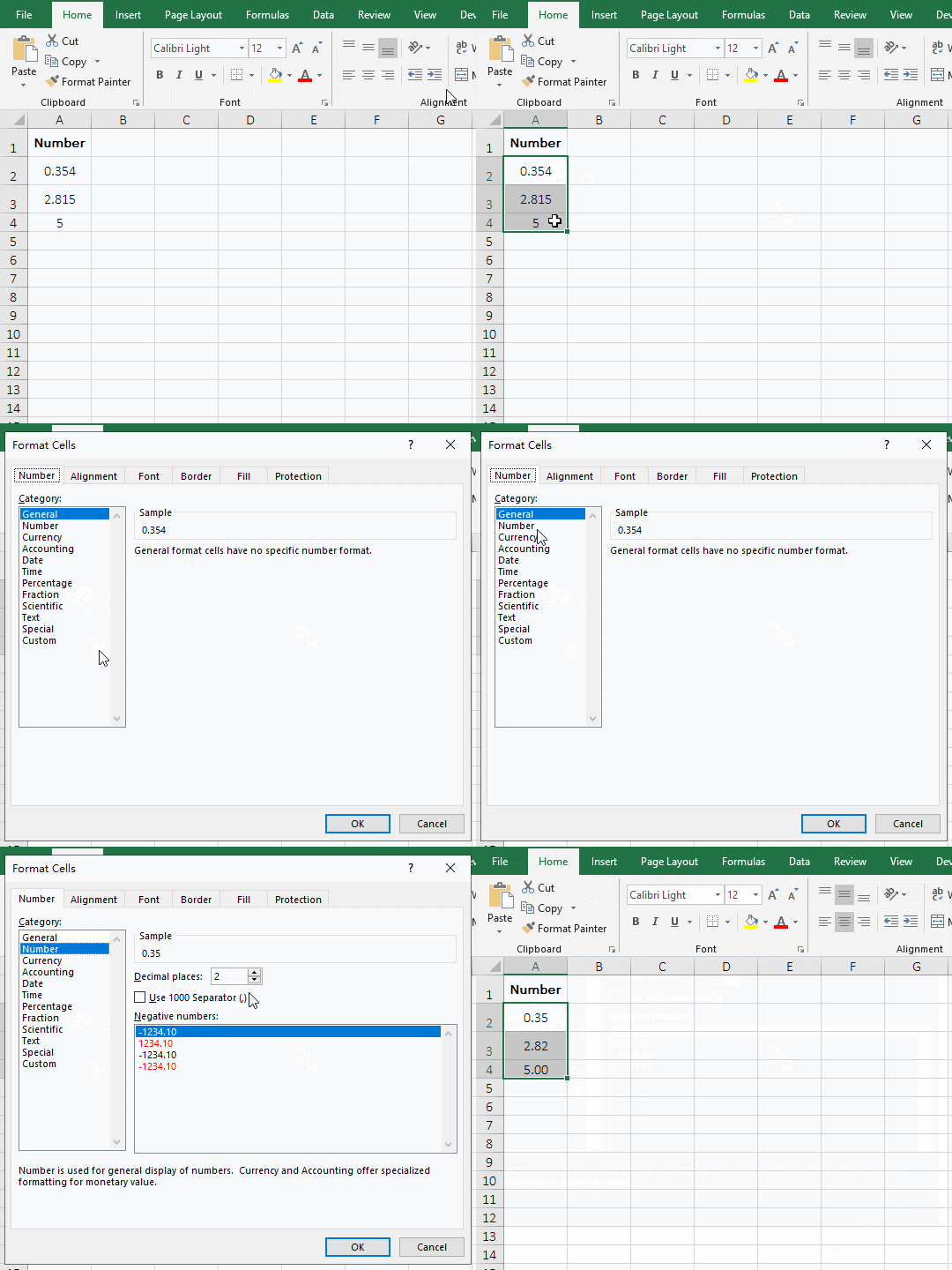
Figure 3

II, Method 2 of how to round numbers in excel: Use the Round function

(I) Round one decimal place

1. If the turnovers is decimal, they are round to one decimal place; if they are integers, return themselves. Double-click cell B2, copy the formula =ROUND(A2,1) to B2, and press Enter, return 68905.9; select A2, click the cell fill handle in the bottom right of A2, and return the remaining turnover are rounded to one decimal place; the operation steps are shown in Figure 4:

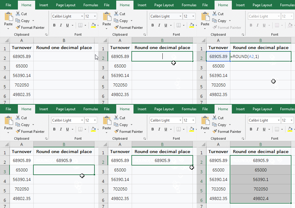
Figure 4

Tip: If you want to round to two decimal places, you only need to change Round's second argument 1 to 2. The formula can be written as follows: =ROUND(A2,2); if you want to round up to the nearest integer, the formula can be written as follows: =ROUND(A2,0); and so on.

2. If you want to round the decimals in the original cell, you can copy the values that have been rounded back to the original cells; the method: Select B2:B6, press Ctrl + C to copy, select A2, and click "Paste" in the top left of the screen, select "Value" under "Paste Values" in the pop-up option, and all the results to be rounded will be copied back to the original cells; the operation steps are shown in Figure 5:

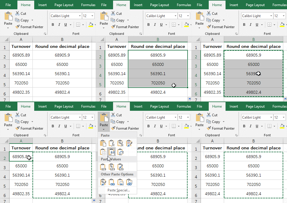
Figure 5

(II) Round one decimal place after averaging

1. If you want to average for the "Advanced Mathematics and English" and their results are round to one decimal place. Double-click cell D2, copy the formula =ROUND(AVERAGE(B2:B18),1) to D2, and press Enter to find their averages and return the result with one decimal place; the operation steps are shown in Figure 6:

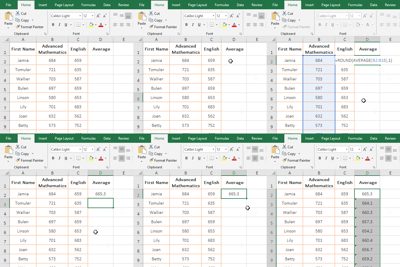
Figure 6

2. Formula description:

AVERAGE(B2:B18) is used to find the average of all the scores in B2:B18, and returns the result to the Round function, then rounds the result to one decimal place with Round function.

III, The extended application of how to round numbers in excel

(I) Rounds automatically

Select the cells to be rounded automatically(such as click A1 to select it, then click A7, select A1:A7), select the "Home" tab, click the drop-down list box in the "Number" group, and select the "Number" from the pop-up options, enter 2.345 in A1, press Enter to automatically round to two decimal places; then enter 5.534 in A2, press Enter to automatically round to two decimal places; the operation steps are shown in Figure 7:

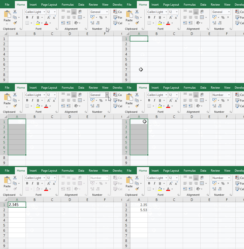
Figure 7

(II) No round

1. If you want to retain two decimal places but not rounded. Double-click cell B1, copy the formula =ROUNDDOWN(A1,2) to B1, and press Enter, return the result 2.34 which the value in A1 is round to two decimal places; select B1, move the mouse to the fill handle in the bottom right of B1, after the mouse changes to a  bold black plus sign, hold down the left button and drag it down to B2, the value in cell A2 round to two decimal places. Double-click cell C1, copy the formula =TRUNC(A1,2) to C1, press Enter to return the same result as B1, drag down to C2, and return the same result as B2. The operation steps are shown in Figure 8:

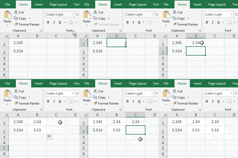
Figure 8

2. Description:

As can be seen from the demonstration, if you only retain two decimal places but not rounded, you can use the two functions RounDown and Trunc, both of which retain only the decimals but not rounded.

(III) The number is greater than or equal to 3, carries 1 to the number before it

1. Double-click cell B1, copy the formula =ROUND(A1+0.001,2) to B1, and press Enter to return 2.64; return 5.54 with dragging down; the operation steps are shown in Figure 9:

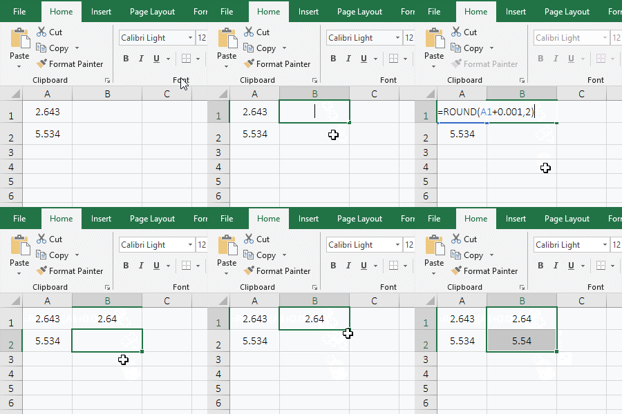
Figure 9

2. Description:

The number is greater than or equal to 3, carries 1 to the number before it is the same as the number is rounded. We can know that before rounding, we add 1 to the number behind the numbers to be rounded the number of decimal places, and then round to the specified decimal place from the demo. For example, first, 2.643 + 0.001 is used, and the result is 2.663, and then it is rounded in the demonstration.

(IV) The number is greater than or equal to 6, carries 1 to the number before it

1. Double-click cell B1 and copy the formula =ROUND(A1-0.001,2) to B1, press Enter to return 2.64. Drag down to B2 and return to 5.54. The operation steps are shown in Figure 10:

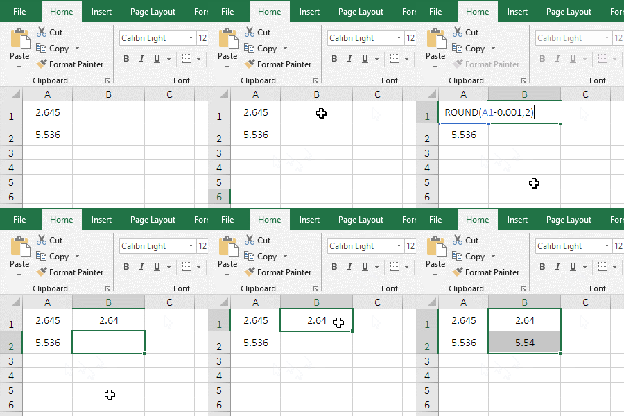
Figure 10

2. Description:

The number is greater than or equal to 6, carries 1 to the number before it is the same as the number is rounded. Before rounding, the number behind the numbers to be rounded the number of decimal places should be reduced by one, and then rounded to the specified decimal place.

(V) Excel rounds to the specified1 multiple

1. If you want to round two decimals to 0.5 times. Double-click cell B2, copy the formula =MROUND(A1,0.5) to B2, press Enter, and return the result 2.5 which 2.64 ia rounded to 0.5 times, and drag down to B2, and return to 6 ; the operation process steps, as shown in Figure 11:

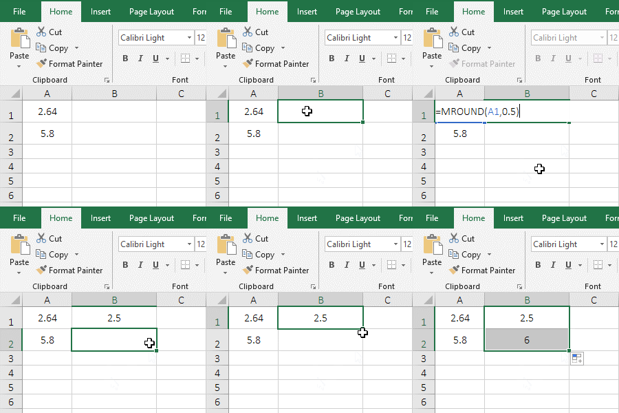
Figure 11

2. Description:

The MRound function is used to round a value to a specified multiple. Its expression is =MROUND(Number,Multiple), the "Number" is the value to be rounded, the "Multiple" is the multiple to be rounded to; if the remainder which the "Number" is divided by the base is greater than or equal to half of the base, the number is rounded away from zero by the MRound function; for example, round 5.8 in A3 to 0.5 times, the remainder of 5.8 divided by 0.5 is 3, and 3 is greater than 0.5, so 5.8 is rounded away from zero, the result is 6.

IV, Excel rounding error(How to fix rounding errors in excel)

(I) Difference 0.1 after rounding

1. Double-click cell D2 and copy the formula =SUM(ROUND(A2,1),ROUND(B2,1),ROUND(C2,1)) to D2, and press enter to return the sum of the three amounts after rounding 896.6; Double-click D3 and copy the formula =ROUND(SUM(A2:C2),1) to D3, press Enter to return the result of rounding up after summing the three amounts. 896.7; operation steps; as shown in Figure 12:

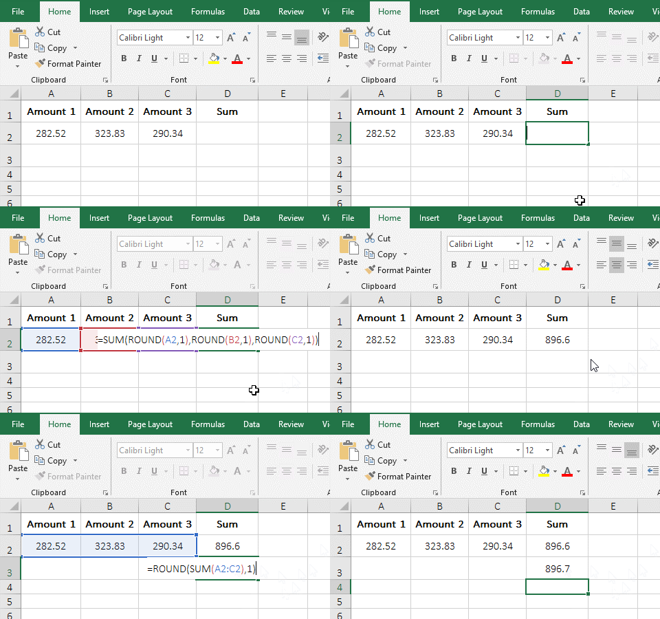
Figure 12

2. Description:

It can be seen from the demonstration that if the three amounts are rounded first and then summed, the amount will be difference 0.1, because the number behind the numbers to be rounded the number of decimal places is less than 5 and discarded; and after the sum is rounded, the three amounts are first added, the numbers behind the numbers to be rounded the number of decimal places of the three amounts are added, they are from less than 5 to 5 or more, and then rounded up to one, so it will be 0.1 more. For example, 0.02 + 0.03 + 0.04 > 0.05 in the demo.

(II) Percentages that are added are not 100% after rounding to

1. Double-click cell C6, copy the formula =SUM(C2:C5) , copy C6, and press Enter to return the result of sum 100%; move the mouse to the fill handle in the bottom right of C6, and after the mouse becomes a bold black plus sign, hold down the left button and drag to the right to return the result of sum of 100.01%; double-click C2, the value inside is calculated by formula, and then double-click D2, the value inside is entered, only 20.2%; select C2, press Ctrl + C to copy, then select C7, click "Paste" in the top left of the screen, and select "Value" under "Paste Values" in the pop-up option, then paste the value in C2 into C7, the result is one long string of numbers; operation steps, as shown in Figure 13:

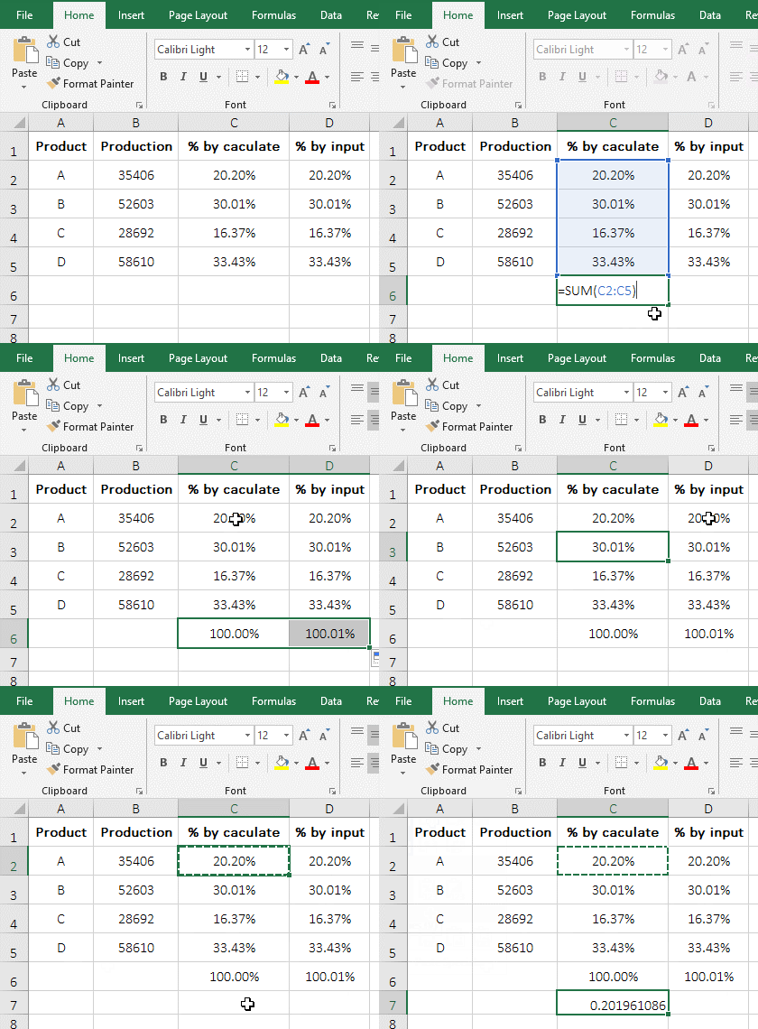
Figure 13

2. Description:

A. The displayed percentages are the same value, but the results of sum are different. The percentage calculated by the formula is exactly 100%, and the percentage to be inputted is 100.01%, which is 0.01% more. Why does this happen?

B. Copy the value in C2 to C7. It can be seen that the percentage obtained by the formula shows the result after rounding. After rounding to the two decimal places, the subsequent digits are not really discarded, but they are hidden, and the percentages to be inputted only have two decimal places to be rounded. All decimal places are added for the former, and only two decimal places are added for the latter. The more decimal places are, the more accurate the sum is. So the sum of the former is exactly 100%, while the latter is 0.01% more. Sometimes the sum of the latter is less than 100%(this will happen if the last digit of the decimal place is less than 5, which is already introduced above).

(III) The amount of each row after rounding is more or less than a few cents, causing the total result to differ too much from the actual value

1. Double-click cell B2, copy the formula =ROUND(A2,0) to B2, and press Enter to return the result 2565 which the salary in A2 is rounded up to. Select B2 and drag down to return 2484; double-click B4, copy the formula =SUM(B2:B3) to B4, press Enter to return the result of sum after the salaries are rounded;

2. Double-click C2 and copy the formula =A2-B2 to C2, press Enter to return to the salary from the salary in A2. Drag down to return to -0.43; double-click D4, copy the formula =SUM(B2:B3,C2:C3) to D4, press Enter to return the subtotalled results of rounded and discarded salaries; the operation steps are shown in Figure 14:

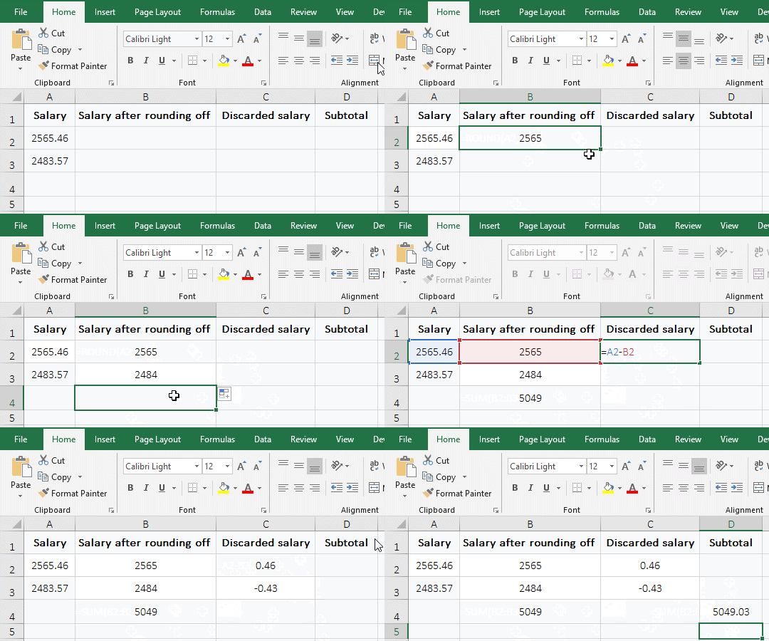
Figure 14

3. Description:

A. Discard salaries with negative signs indicating salaries payable, without negative signs representing deducted salaries.

B. To ensure that the subtotalled results are correct, the discarded results must be calculated into a special column. This can avoid the subtotalled results from being too different from the actual results.