 Office > Excel > Excel 2019 > Content
How to use round function in excel with formula(8 functions, with round off,up,down and even number)
The rounding function is divided into five categories in Excel, which are rounding down to the nearest integer, rounding to, rounding to even, rounding up, and rounding down. There are only two integer parts, namely the Int and Trunc function; one rounding, that is, the Round function; round to the nearest even number is only one, that is, the Even function; there are two for rounding up and down, RoundUp function, Ceiling function and RoundDown function, Floor function, respectively.
There are 8 rounding functions of these five types, only two are used for rounding, that is, Int and Even. Others can round up to the specified number of decimal places, such as Trunc and Round, in addition to integers. Still others can also round values to the specified fractional multiple, such as Ceiling and Floor.
I, Int and Trunc, round a number down to the nearest integer(How to use round function in excel with formula case 1)
(I) Int function
For positive numbers, the Int function only intercepts the integer part and does not round off it; for negative numbers, the Int function advances one regardless of whether the number after the decimal point is greater than or equal to 5; for example:
Select B2, enter the formula =INT(A2), press Enter, return the rounded result 5 of 5.6; select B2, move the mouse to the cell fill handle in the lower right corner of B2, after the mouse becomes bold black plus, double click left button, the returned result of remaining -3.5 and -3.4 is 4; the operation process steps are as shown in Figure 1:
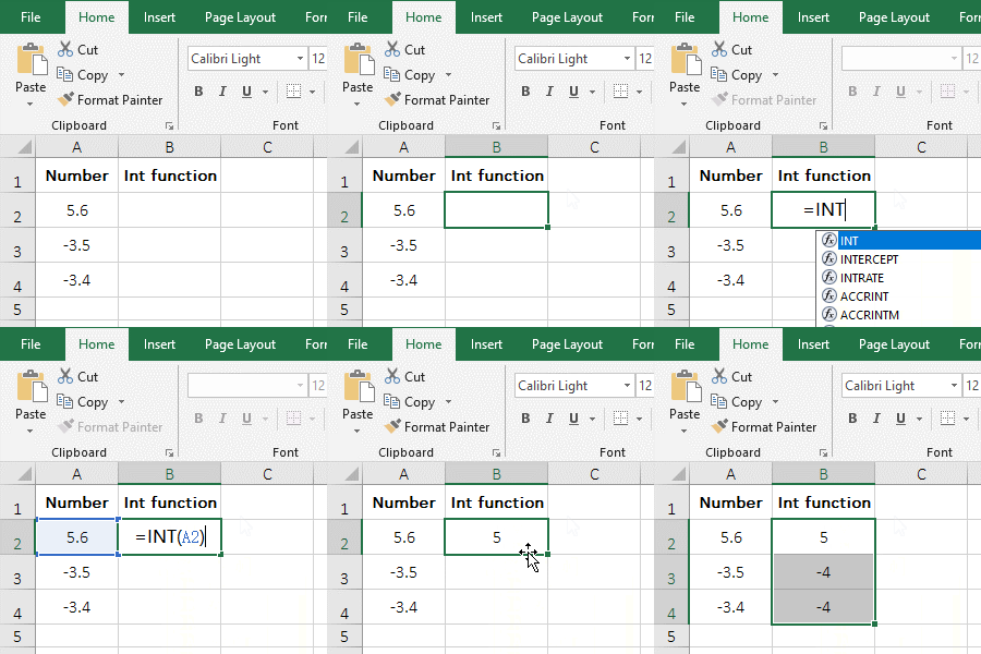
Figure 1
(II) Trunc function
Whether it is a positive or negative number, the Trunc function is not rounded or forwarded. For example:
Double-click cell C2, copy the formula =TRUNC(A2) to C2, press Enter, and the rounded result of 5.6 is also 5; also return the results of -3.5 and -3.4 by double-clicking the cell fill handle of C2, they are all -3; the operation steps are as shown in Figure 2:
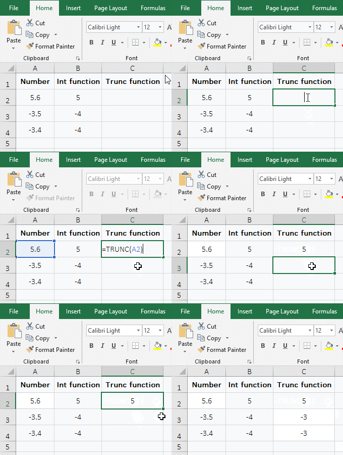
Figure 2
Hint: The the Trunc function can either omit the second argument and set it to 0 when rounded. For example, the above formula can be changed to =TRUNC(A2,0), 0 means to round to 0 decimal places. In addition, the Trunc function can round down to the nearest integer and round to the specified number of decimal places, but in either case, it does not round to. For example: The result which 5.65 is round to 1 decimal place with the formula =TRUNC(5.65,1) is 5.6.
(III) The difference between the Int and Tunc function
The Int function intercepts directly the integer part for the positive number and does not round off it. Whether the number after the decimal point is greater than or equal to 5, it advances one for the negative number; the Trunc function does not round to or advance one for the positive or negative numbers.
II, The function Round, round off(How to use round function in excel with formula case 2)
1. Double-click cell B2, copy the formula =ROUND(A2,0) to B2, press Enter, return to the rounded off result 8; then double-click the cell fill handle of B2 to return the rounded result 9 of 8.5; operation process steps, as shown in Figure 3:
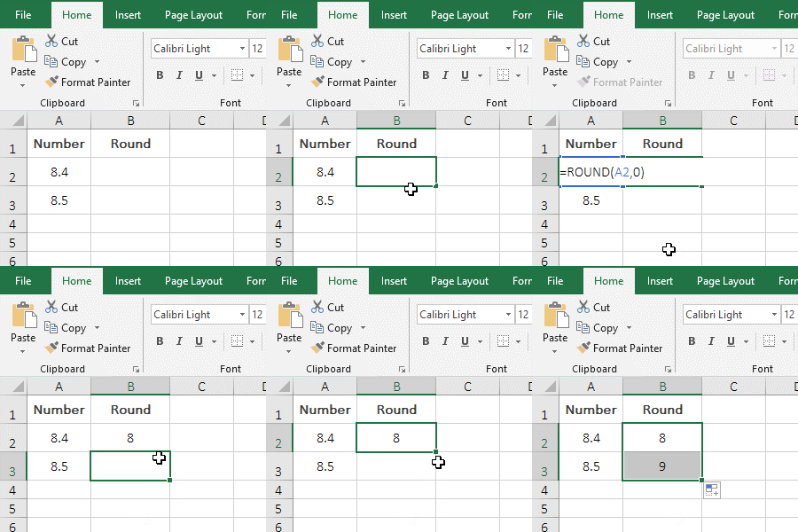
Figure 3
2. Formula description:
The Round function can specify to round to a few decimal places and round the number of digits to the left. When the second argument is 0, the formula =ROUND(A2,0) in the demo, which means that 0 decimal places are rounded to(that is, round a number down to the nearest integer); The second argument is positive, indicating that the specified number of decimal places is rounded to; for example, 8.455 is rounded to 2 decimal places with the formula =ROUND(8.455,2), and the result is 8.46. When the second argument is negative, it means rounding to the left of the decimal point; for example, 85.5 rounds to the left of the decimal point with the formula =ROUND(85.5,-1), and the result is 90, that is, the ones place goes into the tens place.
III, The function Even, round to the nearest even number(How to use round function in excel with formula case 3)
1. Double-click cell B2, copy the formula =EVEN(A2) to B2, press Enter, return the nearest even result 8 of 6.4; also double-click the cell fill the handle of B2 to return the closest even number of the remaining value; the operational steps, as shown in Figure 4:
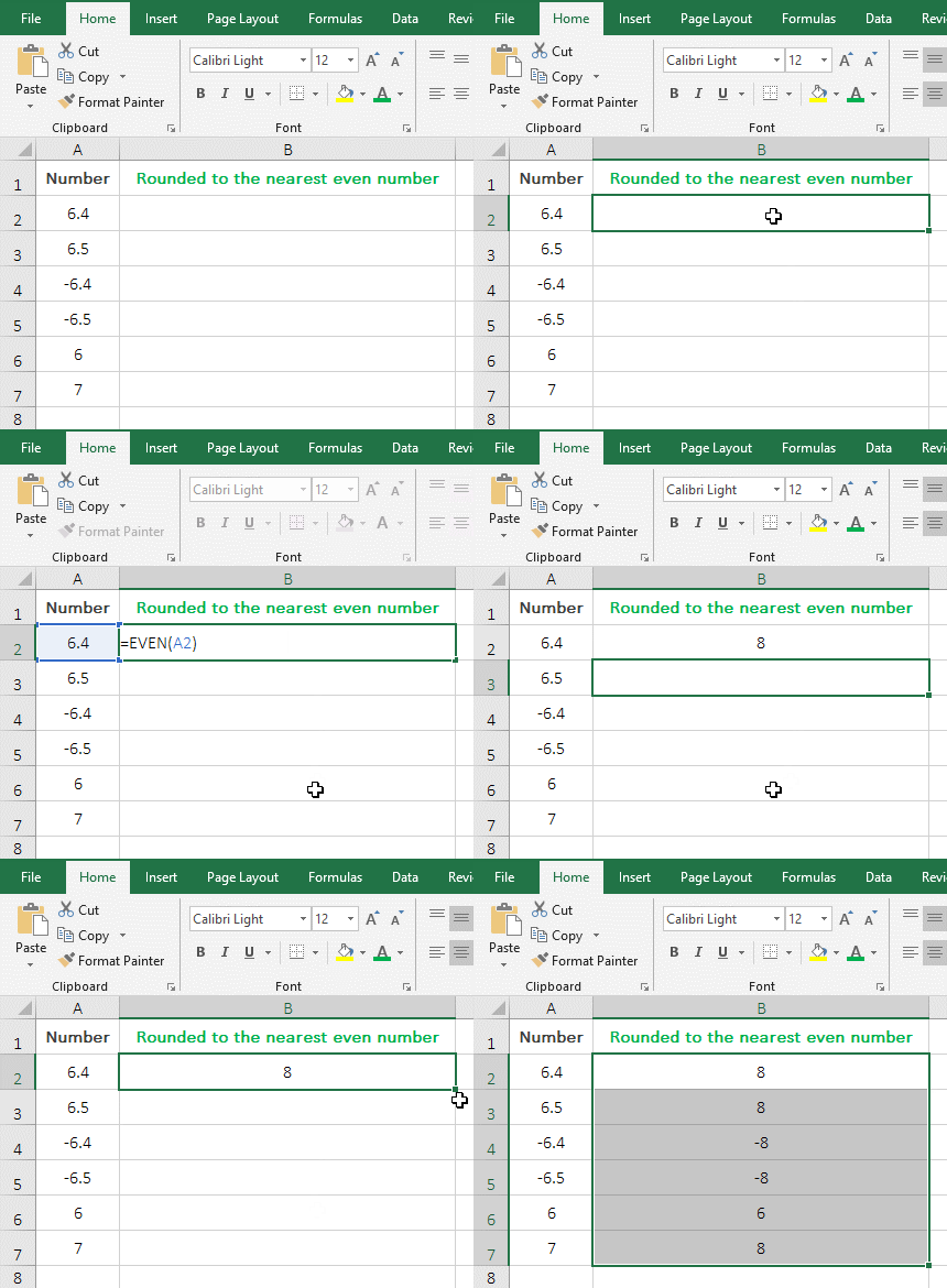
Figure 4
2. Formula description:
The Even function rounds the value in the direction in which the absolute value increases to the nearest even number, and returns itself if the value is already even. Both positive and negative 6.4 and 6.5 return 8 in the demonstration, indicating that Even rounds the positive and negative numbers along the direction in which the absolute value increases to the nearest even number; 6 is an even number, it returns itself; 7 is an odd number, it is rounded to the nearest even number is 8.
IV, RoundUp and Ceiling, both round up(How to use round function in excel with formula case 4)
(I) RoundUp function
1. Double-click cell B2, copy the formula =ROUNDUP(A2,0) to B2, press Enter, and return 3.4 to round up to the nearest integer 4; Double-click the cell fill handle of B2 to return the result of the remaining value; the operation process steps, as shown in Figure 5:
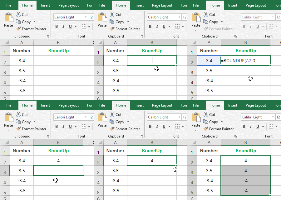
Figure 5
2. Formula description:
When the second argument of the RoundUp function is 0(such as =ROUNDUP(A2,0) in the demo), it is used to round the value away from 0, regardless of whether the value is positive or negative, and not Whether the number after the decimal point is greater than or equal to 5, it is rounded away from 0. For example, 3.4 and 3.5 are rounded to 4, and both -3.4 and -3.5 are rounded to -4 in the demo.
(II) Ceiling function
The expression is: CEILING(Number,Significance), Number is the value to be rounded, and the significance is the multiple to be rounded; the feature is: round the value up to the nearest multiple of the specified base, when the Significance is an integer, the feature is to round the value, which can be divided into three cases, as follows:
(1) The arguments Number and Significance are both positive
1. Double-click B2, copy the formula =CEILING(A2,1) to B2, press Enter, and returns 76 of 75.4 to round up to a multiple of 1; double-click B3, paste the same formula to B3, and change 1 to 2, press Enter, returns 76 of 75.4 round up to a multiple of 2; double-click B4, also paste the same formula to B4, change 1 to 3, return 78 of 75.4 round up to a multiple of 3; then double-click B5, paste the same formula to B5, enter a minus sign(-) before 1, press Enter, return the value error #NUM!; the operation steps are as shown in Figure 6:
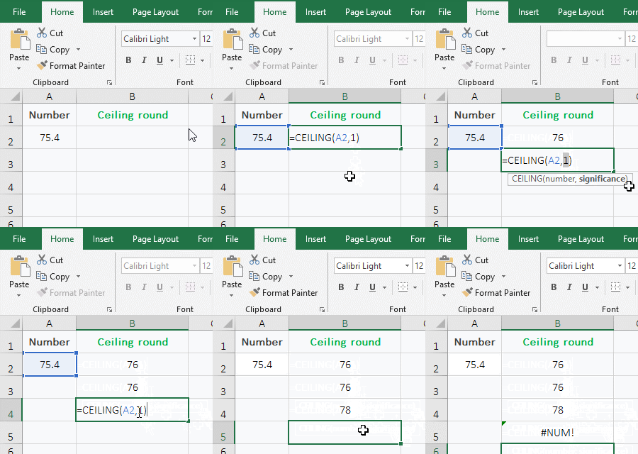
Figure 6
2. Formula description:
As you can see from the demo, when both the argument Number and the Significance are positive, the Ceiling function is rounded up to the nearest multiple of the specified base; for example, both formula =CEILING(A2,1) and =CEILING(A2,2) return 75.4 to round up to a multiple of 1 or 2, respectively, and their result is 76, 76 is a multiple of 1, and is a multiple of 2. However, when the argument Number is a positive number, the Significance cannot be negative, otherwise the #Num! error is returned.
(2) Argument Number is negative and Significance is positive
1. Double-click cell D2, copy the formula =CEILING(C2,1) to D2, press Enter, return to -75; double-click D3, paste the same formula to D3, change 1 to 2, press Enter, return -74; double-click D4, then paste the same formula to D4, change 1 to 3, press Enter, return to -75; operation steps, as shown in Figure 7:
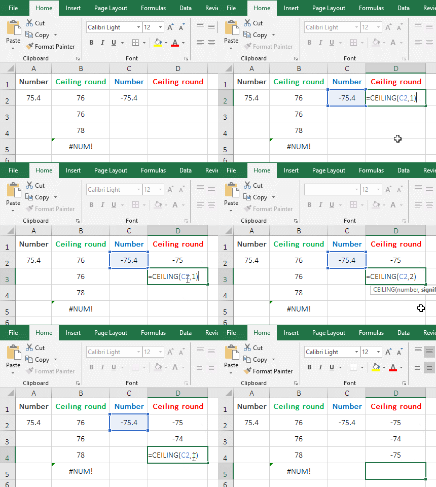
Figure 7
2. Formula description:
When the argument Number is negative and the Significance is positive, the Ceiling function rounds to a multiple of the nearest specified base toward 0. for example, -75.4 is rounded to a multiple of 1, the result is 75; when rounded to a multiple of 2, the result is 74 in the demonstration.
(3) The arguments Number and Significance are both negative
1. Double-click cell F2, copy the formula =CEILING(E2,-1) to F2, press Enter, return to -76; double-click F3, paste the same formula to D3, change 1 to 2, press Enter, return -76; double-click F4, then paste the same formula to F4, change 1 to 3, press Enter, return to -78; the operation steps are as shown in Figure 8:
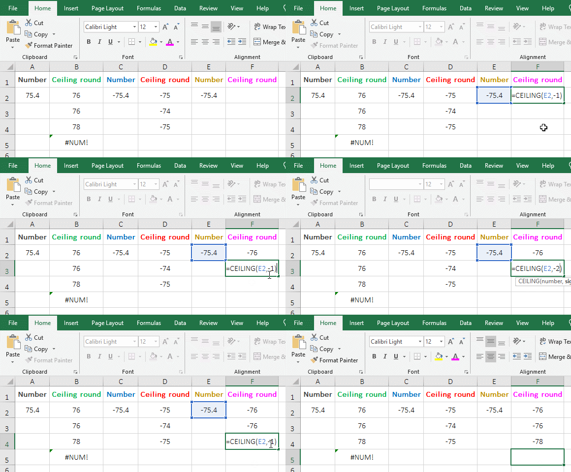
Figure 8
2. Formula description:
When the arguments Number and Significance are both negative, the Ceiling function rounds down to a multiple of the nearest specified base in the direction away from zero. For example -75.4 is rounded to a multiple of -1 and -2, the result is -76; when rounded to a multiple of -3, the result is -78 in the demonstration.
(III) The difference between the RoundUp and Ceiling function
The RoundUp function rounds the positive and negative values away from 0; the Ceiling function rounds the value to a multiple of the specified base.
V, RoundDown and Floor, round down(How to use round function in excel with formula case 5)
(I) RoundDown function
1. Double-click cell B2, copy the formula =ROUNDDOWN(A2,0) to B2, press Enter, return to the rounddowning result 29; double-click the cell fill handle of B2 to return the result of the remaining values; the process steps are shown in Figure 9:
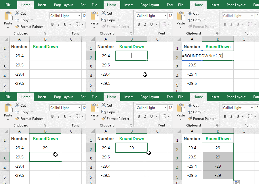
Figure 9
2. Formula description:
When the second argument of the RoundDown function is 0, for example, the formula =ROUNDDOWN(A2,0) is used to round down in the demo. When the value to be rounded is positive or negative, it is rounded toward 0; for example, the rounding result of 29.4 and 29.5 are 29, the rounding result of -29.4 and -29.5 are -29, except that the former is rounded down, and the latter is rounded up.
(II) Floor function
The expression is: FLOOR(Number,Significance), Number is the number to be rounded, Significance is the multiple to be rounded; feature: rounds the value down to the nearest multiple of Significance; when the Significance is positive, the feature is to round the value down to an integer, which can be divided into three cases, as follows:
(1) The arguments Number and Significance are both positive
1. Double-click cell B2, copy the formula =FLOOR(A2,1) to B2, press Enter, return to the result 9 of 9.5 to be rounded down; double-click B3, paste the same formula to B3, and change 1 to 2, press Enter, return to 8; double-click B4, paste the same formula to B4, and change 1 to 3 press Enter, return to 9; then double-click B5, paste the same formula to B5, change 1 to -1, press Enter, return #NUM ! error; operation process steps, as shown in Figure 10:
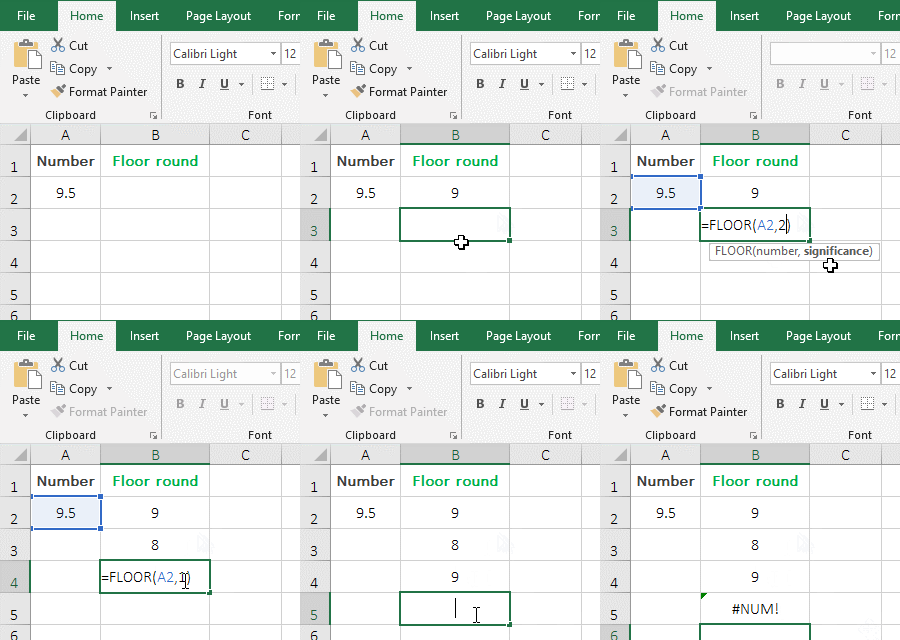
Figure 10
2. Formula description:
When both the argument Number and the Significance are positive, the Floor function rounds down to the nearest multiple of the significance toward 0, for example, 9.5 is rounded down 1 and 3 times, the result is 9 and 9 is the closest to 1 and 3 relative to 9.5, 9.5 is rounded down by 2 times, and the result is 8,8 is also the closest to 2 relative to 9.5.
(2) Argument Number is negative and Significance is positive
1. Double-click cell B2, copy the formula=FLOOR(A2,1) to B2, press Enter, return to -10; double-click B3, paste the same formula to B3, change 1 to 2, press Enter, return -10; double-click B4, then paste the same formula to B4, change 1 to 3, press Enter, return to -12; the operation steps are as shown in Figure 11:

Figure 11
2. Formula description:
When the argument Number is negative and the Significance is positive, the Floor function rounds down to a multiple of the nearest specified Significance in the direction away from zero. For example, -9.5 is rounded down to a multiple of 1 and 2, the result is -10; rounded down to 3 times and the result is -12; they are all away from 0 relative to -9.5.
(3) The arguments Number and Significance are both negative
1. Double-click cell B2, copy the formula =FLOOR(A2,-1) to B2, press Enter, return to -9; double-click B3, paste the same formula to B3, change -1 to -2, press Enter, return -8; double-click B4, paste the same formula to B4, change -1 to -3, press Enter, return to -9; the operation steps, as shown in Figure 12:
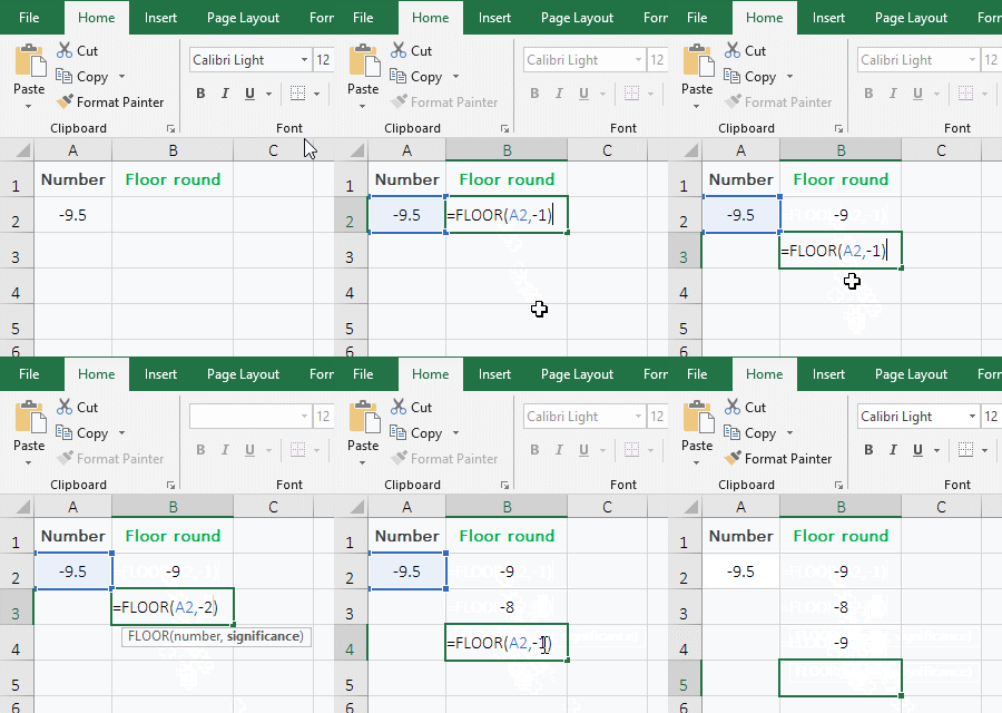
Figure 12
2. Formula description:
When the arguments Number and Significance are both negative, the Floor function is rounded to the nearest multiple of Significance toward 0. For example, -9.5 is rounded to a multiple of -1 and -3, the result is -9; rounded to a multiple of -2, the result is -8; the rounding result is toward 0 and is the number closest to -1, -2, and -3, relative to -9.5.
(III) The difference between RoundDown and Floor function
When the RoundDown function is used for rounding, the value to be rounded is rounded toward 0 whether it is positive or negative. The Floor function rounds the value to a multiple of the specified base.
-
Related Reading
- Excel CountA and CountBlank function usage examples(
- 8 examples of Excel Match function, include it and S
- How to use offset function in excel, include it and
- Excel SumProduct function(multiple criteria, with if
- Excel left function usage(8 examples, with Sum+Value
- How to round numbers in excel and fix rounding error
- How to use Average function in excel(combine with if
- Excel round to 2 decimal places and no display 0, or
- How to use Excel address function(7 examples, with I
- Excel SumIf function with ?/*, Average and array mul
- How to use Excel subtotal function(combine it with O
- How to use excel aggregate function(ignore error val