Excel AverageIfs function usage(7 examples, include multiple criteria ane two dates)

The AverageIfs function is used to meet two or multiple criteria averages in excel, while the AverageIf function is only used for one criteria for averaging. The AverageIfs function must have at least one criteria, and no more than 127 criteria. The criteria is "And" relationship. In addition, it is a new addition to Excel 2007 and can only be used in Excel 2007 or later.

Using the AverageIfs function to multiple criteria averaging often encounters a divisor to 0 error, empty cell processing, valid and neglected logical values, criteria with expressions, functions, and wildcard question marks? and asterisks *, the shape and size of criteria range and average range must be the same, and Excel averageifs multiple criteria in the same column. These problems are all accompanied by specific examples or detailed descriptions.

I, The syntax of Excel AverageIfs function

1. Expression: AVERAGEIFS(Average_Range, Criteria_Range1, Criteria1, [Criteria_Range2, Criteria2], ...)

2. Description:

A. Criteria_Range1 and Criteria1 form a Criteria_Range/Criteria pair, and the AverageIfs function cannot exceed 127 Criteria_Range/Criteria pairs at most.

B. If Average_Range is all null, text, or a value that cannot be converted to a numeric value, the AverageIfs function will return a divisor to 0 error #DIV/0!; if there is no cell that meets the Criteria, the AverageIfs function also returns #DIV/0 ! error.

C. An empty cell in the Criteria_Range, which the AverageIfs function treats as 0. If the range contains a logical value True or False, True is converted to 1, and False is converted to 0.

D. Criteria can be numbers, characters(such as "qualified"), expressions(such as ">=1" or ">="&1) and references to cells. In addition, wildcard question marks(?) and asterisks(*) can also be used in the Criteria. The question mark indicates any character, the asterisk indicates one or a string of characters. If you want to find a question mark or an asterisk, you need to add an escape character ~ before them, such as ~?, ~*.

E. AverageIfs function requires that each Criteria_Rang must be the same size and shape as Average_Range, and the AverageIf function can be different. For example, if Criteria_Rang is A2:A100 and Average_Range is B2:B100, they are the same size and shape; if Average_Range is B3:B100, their size and shape are different.

II, The examples of Excel AverageIfs function

(I) Return the average of two Criteria

1. If you want to sell the average sales of "Women's clothing" in New York. Double-click the cell E9, copy the formula =AVERAGEIFS(E2:E8,B2:B8,"Women's clothing",C2:C8,"New York") to E9, press Enter, return to the average result 643; operation steps, such as Figure 1 shows:

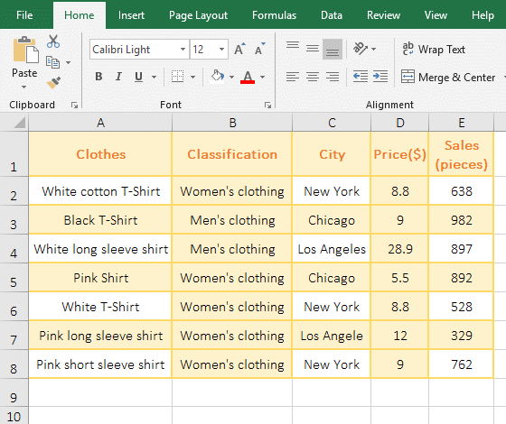
Figure 1

2. Formula =AVERAGEIFS(E2:E8,B2:B8,"Women's clothing",C2:C8,"New York") explanation:

E2:E8 is the Average_Range; B2:B8 is the Criteria_Range1, "Women's clothing" is the Criteria1; C2:C8 is the Criteria_Range2, and "New York" is the Criteria2; the meaning of the formula: Find all the "Women's clothing" in B2:B8, then find all the clothes that are sold in "New York" in C2:C8, then return the average of the two Criteria in E2:E8.

(II) Return divisor is 0 error #DIV/0!

1. Double-click the cell A8, copy the formula =AVERAGEIFS(A2:A7,C2:C7,">=3") to A8, press Enter, return the divisor to 0 error #DIV/0!; then double-click D8, copy the Formula =AVERAGEIFS(D2:D7,C2:C7,">=10") to D8, press Enter, and return to divide to 0 error; the operation process steps, as shown in Figure 2:

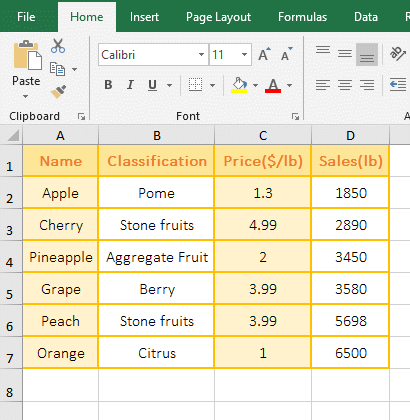
Figure 2

2. The Average_Range is A2:A7 in the formula =AVERAGEIFS(A2:A7,C2:C7,">=3"), although there are records in C2:C7 that meet the Criteria, but the value in A2:A7 is all text, so returns a divisor to 0 error. D2:D7 in the formula =AVERAGEIFS(D2:D7,C2:C7,">=10") is all numeric, but C2:C7 does not have a record that meets the Criteria, so the divisor is also returned as 0 error.

(III) Logic value True or False Valid and ignored

1. Double-click the cell A7 cell, copy the formula =AVERAGEIFS(A1:A6,B1:B6,TRUE) to A7, press Enter, return to the average result 6; the operation steps are as shown in Figure 3:

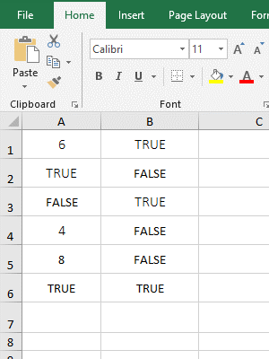
Figure 3

2. Formula =AVERAGEIFS(A1:A6,B1:B6,TRUE) Averages in A1:A6, Criteria is TRUE in B1:B6, and only B1, B3, and B6 are satisfied, the values in A2, A3 and A6 are TRUE, FALSE and TRUE, respectively, and the average result is 6, indicates that A2, A3 and A6 are not included in the average, that is, the logical value is ignored in the Average_Range; and the records that the logical value are TRUE can be selected in B1:B6, indicates that the logical value is valid in the Criteria_Range.

(IV) Use wildcards ? or * in Criteria

1. If you want to average for the Sales of Clothes whose "No." start with "NS" and have only thirteen characters. Double-click the cell F11, copy the formula =AVERAGEIFS(F2:F10,A2:A10,"NS*",B2:B10,"?????????????") to F11, press Enter, return to the average result 812.5; the process steps are shown in Figure 4:

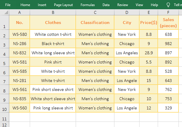
Figure 4

2. Formula =AVERAGEIFS(F2:F10,A2:A10,"NS*",B2:B10,"?????????????") explanation:

F2:F10 is the Average_Range; "A2:A10,"NS*"" is the first Criteria_Range/Criteria pair, which means that all clothing starting with "NS" are found in A2 to A10, and "*" after "NS" means any one Or multiple characters. "B2:B10,"?????????????"" is the second Criteria_Range/Criteria pair, meaning to find all the Clothes with only thirteen characters in B2:B10. When executing, the clothes that meet the first Criteria are found, then match the found clothes to the second Criteria, and finally return the clothes that meets the two Criteria, and then calculate the average of these clothes in the F column.

(V) The same range is simultaneously Average_Range and Criteria_Range

1. If you want to average for the Sales of Clothes Whose "Classification" equal "Women's clothing" and Sales are greater than 0. Double-click the cell E9, copy the formula =AVERAGEIFS(E2:E8,C2:C8,"Women's clothing",E2:E8,">0") to E9, press Enter, return to the average result 564; As shown in Figure 5:

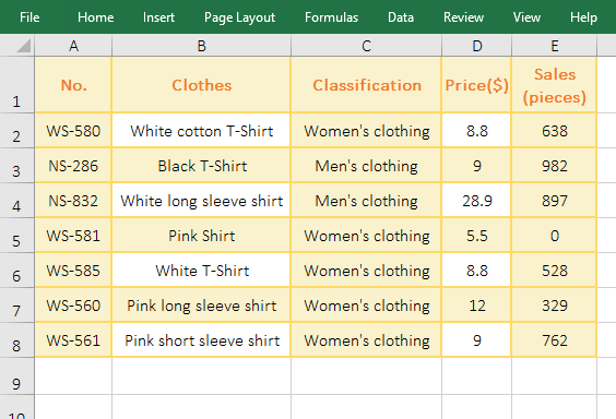
Figure 5

2. E2:E8 in the formula is both the Average_Range and the range of the second Criteria ">0", indicates that the same range can be both average and Criteria Range.

Hint: If the Average_Range has empty cells and you don't want to count them into average, you can exclude them with the Criteria ">0".

(VI) Excel averageifs multiple criteria in the same column

1. If you want to average for the Sales of Clothes whose price is between 10 and 30. Double-click the cell E11, copy the formula =AVERAGEIFS(E2:E10,D2:D10,">=10",D2:D10,"<=30") to E11, press Enter to return to the average result 656; the process steps are shown in Figure 6:

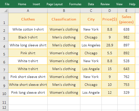
Figure 6

2. The two Criteria_Range are D2:D12 in the formula =AVERAGEIFS(E2:E10,D2:D10,">=10",D2:D10,"<=30"), which means that the Clothes whose price are greater than or equal to 10 and less than or equal to 30 are found in D2:D10, and then average them in the E column.

(VII) Excel Averageifs between two dates

1. If you want to average for the Sales of Clothes whose Date is between 2018/9/10 and 2018/9/11. Double-click the cell D12, copy the formula =AVERAGEIFS(D2:D11,B2:B11,">=2018/9/10",B2:B11,"<=2018/9/11") to D12, press Enter, return the result 805; the process steps are shown in Figure 7:

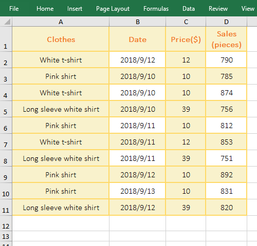
Figure 7

2. The both Criteria_Range are B2:B11, in the formula =AVERAGEIFS(D2:D11,B2:B11,">=2018/9/10",B2:B11,"<=2018/9/11"); when dates coincide with compositions greater than or equal to, you can write them together from the first Criteria ">=2018/9/10". The mean of formula that the Clothes whose Date is between 2018/9/10 and 2018/9/11 in B2:B11, and then average them in the D column.