How to use Average function in excel(combine with if, sum, month in formula)

The Average function is used to return the average of numeric values in excel. It must have at least one value with a maximum of 255 values. If you want to average the text or logical values, you need to use the AverageA function.

The Average function can be averaged with some functions, such as the Average + If combination to achieve the interlaced (or specified condition) for averaging, the Average + If + Int + Left + Find combination to average quarterly, and the Average + Year combination to average annual, Average + Month combination to average monthly.

I, Syntax of Average function in excel

1. Average formula in excel: =AVERAGE(Number1, [Number2], ...)

2. Description:

A. Number can be a number, an array, a name containing a number or numbers, and a range. There must be at least one Number and at most 255 Numbers.

B. If Number is a text that can be converted to a numeric value (such as "1"), the Average function will automatically convert it to a numeric value; if Number is a text that cannot be converted to a numeric value (such as "one" or "A"), the Average function will return the value error #VALUE!. If there is text in the referenced cell (the cell format is text); they will be ignored. If the array has text, the value that can be converted to the number will be counted as an average, and those that cannot be converted to a number will be ignored. If there is an error value in argument Number, an error is returned.

C. If there are 0 or null cells in the referenced cells, 0 will be counted as averaging, and null values will not be counted as averaging.

D. If the referenced cells have logical values True or False, they are ignored; if Number is an array and contains logical values, True is converted to 1, and False is converted to 0.

E. If you want to calculate the logical value in the referenced cell and the value of the cell format as text, you need to use the AverageA function.

II, The examples of Average function in excel

(I) How to create an average formula in excel

1. Double-click the cell B1, copy the formula =AVERAGE(A1:A3) to B1, press Enter, return to the averaging result 7; the operation steps are as shown in Figure 1:

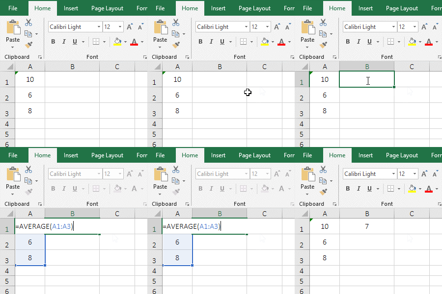
Figure 1

2. There are three values in A1:A3, and the average result is 7. It means that 10 in A1 is not counted as averaging, and there is a small green triangle in the upper left corner of A1, indicating that the cell format of A1 is text, and the function Average does not count the numbers in text format as averaging.

(II) There is text in the array

1. Double-click the cell A1, copy the formula =AVERAGE(4,"6",8) to A1, press Enter, return to the average result 6; double-click A1, change 6 to "one", press Enter. return value error #VALUE!; Operation process steps, as shown in Figure 2:

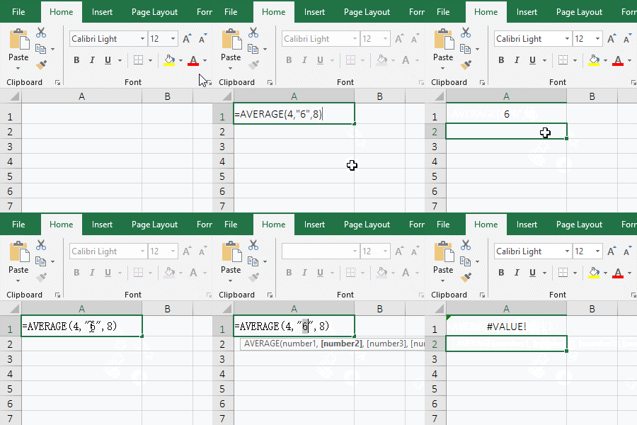
Figure 2

2. The formula = AVERAGE (4,"6",8) returns 6, indicating that the text "6" is included in the averaging; and after changing "6" to "one", an error is returned, indicating that there are the texts that cannot be transferred number in the argrments, the Average function returns an error.

(III) There are 0 and incorrect values in the referenced cells

1. Double-click the cell B1, copy the formula =AVERAGE(A1:A4) to B1, press Enter, and return the value error #VALUE!; select A1, delete the content, and the value of B1 becomes divisor 0 Error #DIV/0!; then delete the contents in A2, the value in B1 becomes 0; the operation process steps, as shown in Figure 3:

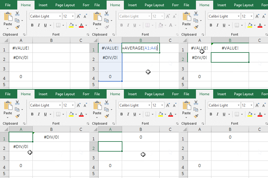
Figure 3

2. From the above operation, the Average function returns an error when there is an error value in the referenced cells; the empty cell in the referenced cells is ignored, and 0 is included in the averaging.

(IV) There are logical values True or Falsea in the referenced cells or array

1. Double-click the cell A3, enter the formula =AVERAGE(A1:A2), press Enter, return the divisor to 0 error #DIV/0!; double-click A4, copy the formula=AVERAGE(TRUE,FALSE) to A4, press Enter, returns to the average value 0.5; the operation steps are as shown in Figure 4:

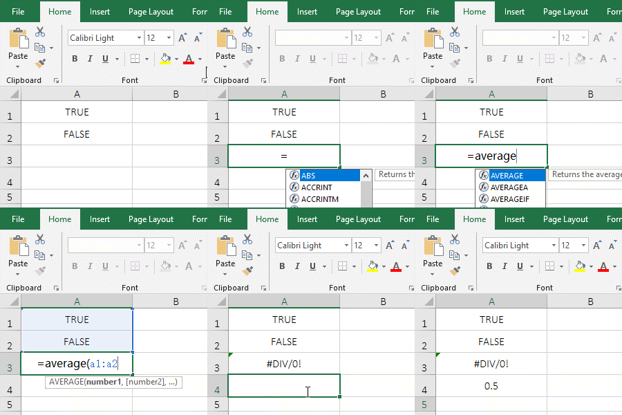
Figure 4

2. The formula = AVERAGE(A1:A2) and =AVERAGE(TRUE,FALSE) are both averaging True and False, but the former returns the error and the latter can return the correct value, indicating that the logical value is in the cell, they are ignored by the Average function, and they are counted as averaging as arguments to the Average function.

III, Extension use case o Average function in excel

(I) Average + If function combination to achieve interlaced averaging(or average according to specified conditions)

1. If you want to get the average of the sales of "Women's clothing and Men's clothing" separately. Double-click the cell C11, copy the formula =AVERAGE(IF(C$2:C$8=B11,E$2:E$8,"")) to C11, press Ctrl + Shift + Enter to return to the averaging result 629.8; Move the mouse to the cell fill handle in the lower right corner of C11, after the mouse becomes the bold black plus, hold down the left button and drag down to return the average of Sales of all "Men's clothing"; the operation steps are as shown in Figure 5:

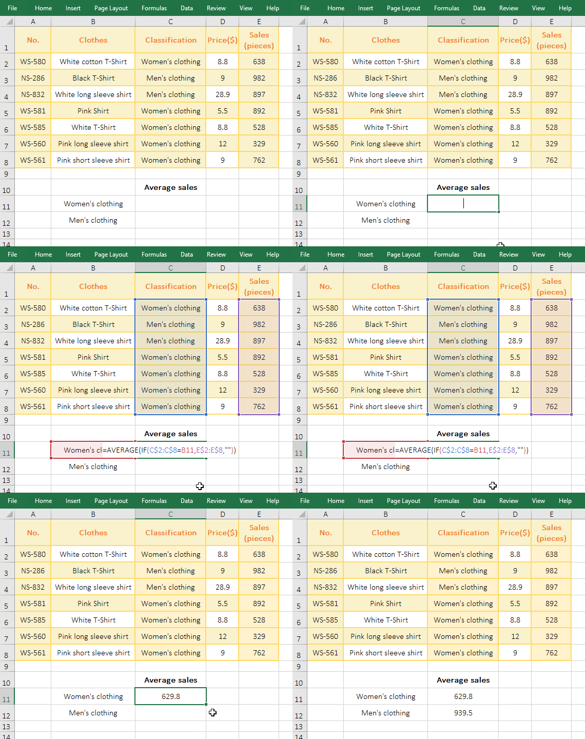
Figure 5

2. The formula =AVERAGE(IF(C$2:C$8=B11,E$2:E$8,"")) description:

A. C$2 is a relative reference to the column, absolute reference to the row, when dragging down, C2 will not become C3, C4, etc.; C$8, E$2, E$8 and C$2 are the same meaning; and A12 is are relative references for column and Rows, when dragging down, A12 will change to A13; any addition of $ before the column or row means absolute reference.

B. C$2:C$8 returns all the values in C2 to C8 as an array, then the condition C$2:C$8=B11 of If becomes {"Women's clothing"; "Men's clothing"; "Men's clothing";"Women's clothing"; "Women's clothing"; Women's clothing; "Women's clothing"}="Women's clothing"; then, take each element from the array and compare it with "Women's clothing", if they equal, returns True, otherwise returns False; for example: take out "Women's clothing" for the first time, it is equals to "Women's clothing", so it returns True; "Men's clothing" is taken out for the second time, it is not equal to "Women's clothing", so it returns False; the others and so on, and finally returns {TRUE; FALSE; FALSE ;TRUE; TRUE;TRUE;TRUE}.

C. Then IF(C$2:C$8=B11,E$2:E$8,"") becomes IF({TRUE; FALSE; FALSE ;TRUE; TRUE;TRUE;TRUE},E$2:E$8,""), Then take each element from the condition array of If, if it is TRUE, return the element corresponding to D$2:D$8, otherwise return ""; for example: take TRUE fpr the first time, return D2; take FALSE for the second time , return ""; finally returned {638;"";"";892;"";528;329;762}.

D. The formula becomes =AVERAGE({638;"";"";892;"";528;329;762}), averaging the elements in the array finally, and returns 629.8.

Tip: In addition to the implementation of the Average + If function, you can also use the AverageIf function to achieve, that is, =AVERAGEIF (C2:C8, B11, D2:D8).

(II) Average + If + Int + Left + Find function combination to average quarterly(not necessarily three months per quarter)

1. If you require an average sales per quarter. Double-click the cell E2, copy the formula =AVERAGE(IF((INT(A$2:A$11)>(3*D2-3))*(INT(A$2:A$11)<=3*D2),B$2:B$11,"")) to E2, press Ctrl + Shift + Enter, return to the average result 4514.33; select E2, move the mouse to the lower right corner of E2, double-click after the mouse becomes the bold black plus, returs the average sales of other quarters, the operation process steps, as shown in Figure 6:

Figure 6

2. Formula =AVERAGE(IF((INT(A$2:A$11)>(3*D2-3))*(INT(A$2:A$11)<=3*D2),B$2:B$11,"")) explanation:

A. A$2:A$11 returns the month in A2:A11 as an array, ie {"1";"2";"3";"4;"5";"6";"7";"8";"9";"10"}.

B. Then INT(A$2:A$11) becomes INT({"1";"2";"3";"4;"5";"6";"7";"8";"9";"10"}), further calculations round up each element in the array, and finally return {1;2;3;4;5;6;7;8;9;10}.

C. D2 is 1, substituting it into 3*D2-3 to get 0, then substituting it into 3*D2 to get 3; the formula becomes =AVERAGE(IF({1;2;3;4;5;6;7; 8;9;10}>0)*({1;2;3;4;5;6;7;8;9;10}<=3), B$2:B$11,"")), and then, take each element from the conditional array of if, it is compared with 0; if it is greater than 0, it returns True, otherwise it returns False, and finally returns {TRUE;TRUE;TRUE;TRUE;TRUE;TRUE;TRUE;TRUE;TRUE;TRUE}.

Then take each element from the second conditional array of if, it is compared with 3, if it is less than or equal to 3, it returns True, otherwise it returns False, and finally returns {TRUE;TRUE;TRUE;FALSE;FALSE;FALSE;FALSE;FALSE;FALSE;FALSE}.

D, then the formula becomes =AVERAGE(IF({TRUE;TRUE;TRUE;TRUE;TRUE;TRUE;TRUE;TRUE;TRUE}*{TRUE;TRUE;TRUE;FALSE;FALSE;FALSE;FALSE;FALSE;FALSE} , B$2: B$10, "")), then multiply the corresponding elements of the two arrays. When multiplied, True is converted to 1, and False is converted to 0.

E. The formula becomes =AVERAGE(IF({1;1;1;0;0;0;0;0;0}, B$2:B$11,"")), and then, take out each element from the conditional array of If, if it is True, returns the corresponding element in B2:B11, otherwise return ""; for example: take the first element 1 from the conditional array for the first time, because it is True, it returns 5253; takes out the second Element 1 for the second time, return 3643; others and so on, and finally return {5253;3643;4647;"";"";"";"";"";"";""}.

F. The formula becomes =AVERAGE({5253;3643;4647;"";"";"";"";"";"";""}), and finally the elements in the array are averaged and the result is 4514.33.

(III) Year and month average

(I) Average + If + Year function combination to average annual

1. If there is a sales table for 2019, the annual average sales is required. Double-click the cell E2, copy the formula =AVERAGE(IF(YEAR(A$2:A$362)=D2,B$2:B$362,"")) to E2, press Ctrl + Shift + Enter to return to the averaging result 536.92; operation process steps, as shown in Figure 7:

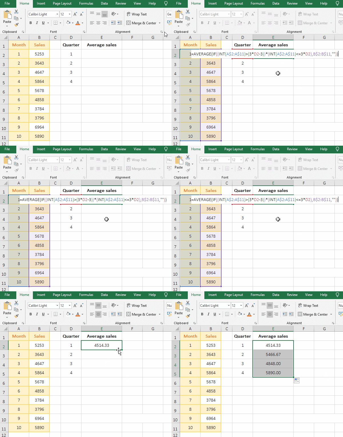
Figure 7

2. Formula =AVERAGE(IF(YEAR(A$2:A$362)=D2,B$2:B$362,"")) description:

A. YEAR(A$2:A$362) returns the year in A2:A362 as an array, ie {2019;2019;...;2019}.

B. Then YEAR(A$2:A$362)=D2 becomes {2019;2019;...;2019}=D2, and then take out each 2019 from the array, it is compared with D2(ie 2019), since they are all equal, so returns True all, ie {TRUE;TRUE;...;TRUE}.

C. The formula changes = AVERAGE(IF(TRUE;TRUE;...;TRUE}, B$2:B$362,"")), then, take each element from the conditional array, if it is true, return the corresponding value in B2:B362, otherwise returns ""; since the condition array is all true, all values in B2:B362 are returned as an array, ie {569;486;...;678}.

D. The formula becomes =AVERAGE({569;486;...;678}), and finally the values in the array are averaged and the result is 536.92.

Tip: If the table has data for different years at the same time, you can also use the above formula to request the average of that year, just write the specific year to D2.

(II) Average + If + Month function combination to achieve monthly average

1. If you require an average sales volume from January to December. Double-click the cell D4, copy the formula =AVERAGE(IF(MONTH(A$2:A$362)=D4,B$2:B$362,"")) to D4, press Enter, return to the average 533.81 of January; Use the method of double-click the cell fill handle to retrun the average sales volume of the remaining months; the operation process steps are as shown in Figure 8:

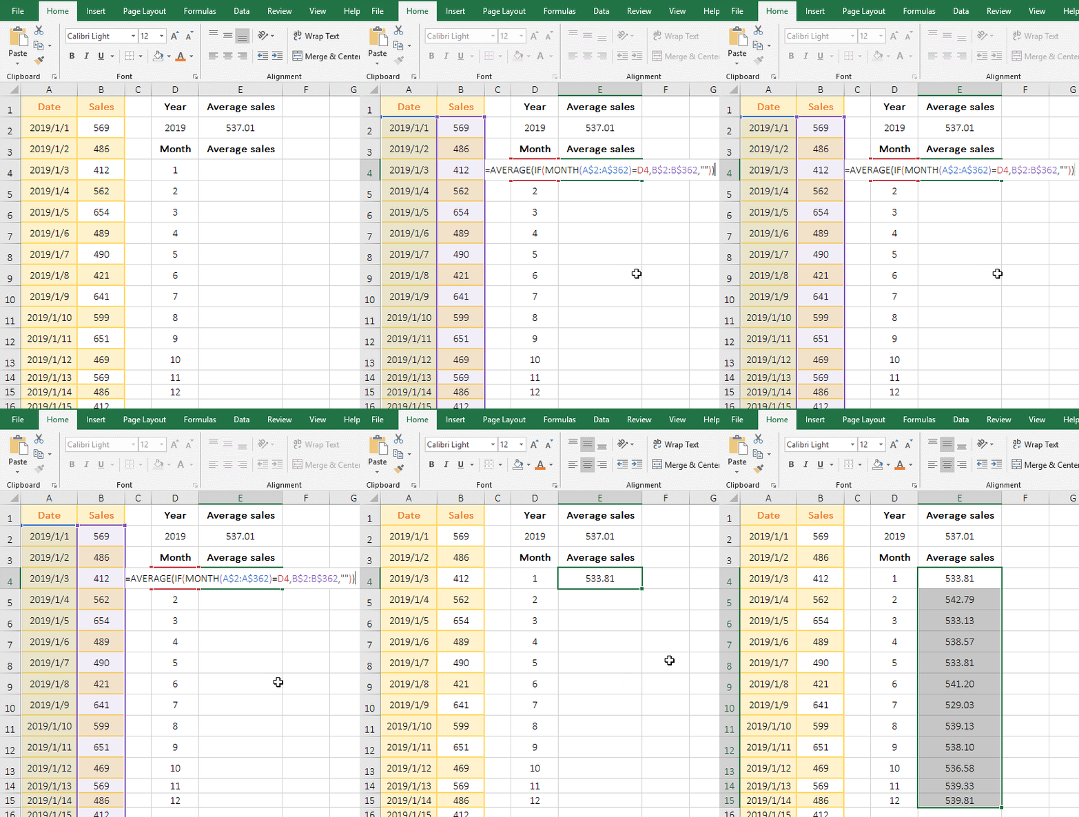
Figure 8

2. Formula =AVERAGE(IF(MONTH(A$2:A$362)=D4,B$2:B$362,"")) description:

The formula is the same as the annual average formula. The difference is that MONTH(A$2:A$362) is used to take the month of the date from A2 to A362; for example, the first time is 1 month of 2019/1/1 in A2.