 Office > Excel > Excel 2019 > Content
8 examples of Excel Match function, include it and Sum, OffSet, Indirect combination to extract data
The Match function is used to return the relative position of the lookup value in the reference cell in Excel. It has three arguments, the first argument is the LookUp_Value, the second is the LookUp_Array, and the third is the Match_Type; the Match_Type can be set to exact match and fuzzy match, where the fuzzy match needs to be sorted.
The Match function is often used in combination with the Index, Sum, OffSet, and Indirect functions. The combination of Index + Match or Indirect + Match can return multiple values in the cells at the intersection of the row and column (that is, extract data), and the OffSet + Match combination can return the value that is corresponded to the minimum value that is greater than or equal to the LookUp_Value in a column, and the Sum + OffSet + Indirect + Match combination implements dynamic cross-table summation for the changed region. The following are 8 examples(multiple match formula in excel) of how to use the Match function.
I, Excel Match function syntax
1. Expression: MATCH(LookUp_Value, LookUp_Array, [Match_Type])
2. Description:
(1) Match_Type is optional. It has three values, which are 1, 0, and -1. If Match_Type is omitted, the default is 1.
A. If Match_Type is omitted or taken 1, finds the maximum value that is less than or equal the LookUp_Value, and the values in LookUp_Array are sorted in ascending order, otherwise an incorrect value may be returned.
B. If Match_Type takes 0, it finds the first value that is exactly equal to the LookUp_Value. The LookUp_Array does not need to be sorted.
C. If Match_Type takes -1, finds the minimum value greater than or equal to the LookUp_Value, the values in LookUp_Array are sorted in descending order, otherwise it may return an incorrect value.
(2) When Match_Type is 0 and the LookUp_Valu is text, the wildcard characters "question mark(?) and asterisk(*)" can be used in the lookup value; the question mark indicates any character, and the asterisk indicates any one or a string of characters; To find question marks or asterisks, you need to precede them with an escape character(~); for example: the search "question mark(?)" should be written like this: ~?, the search asterisk should be written like this: ~*.
(3) If the Match function cannot find a value, it will return the error value #N/A; in addition, when finding text, the Match function is not case sensitive.
II, The use examples of Excel Match function
(I)Match_Type omitted or taken 1
1. If you want to find the position of the "First Name" as "Babily" in the employee table. Double-click the cell A10, copy the formula =MATCH("Babily", A2:A9) to A10, press Enter, return the error value #N/A; select A2:A9, select the "Data" tab, click " Ascending" icon(A→Z), open the "Sort Warning" window, keep the default option "Extended the selecting", click "Sort", then the table will be sorted in ascending order by "First Name", the value in A10 was changed to 2; double-click A10, add the third argument 1 to the formula, press Enter, also return 2; the operation steps, as shown in Figure 1:
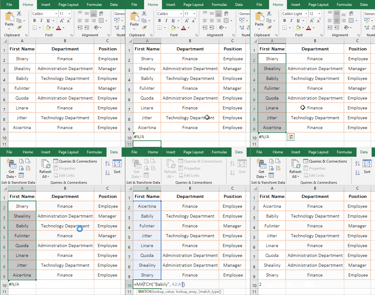
Figure 1
2. Formula description:
A."Babily" is the LookUp_Value in the formula =MATCH("Babily", A2:A9), A2:A9 is the LookUp_Array, it omits the argument Match_Type, when the A column is not sorted in ascending order, the error value is returned #N/A, when sorted, can return the position of "Babily" in A2:A9. When the Match_Type(set to 1) is added to the formula, it also returns 2 indicating that the Match_Type is omitted or 1 is taken, the LookUp_Array must be sorted in ascending order and find the maximum value that is less than or equal to the Lookup_Value.
B. In addition, the position of the LookUp_Value in the LookUp_Array starts from the selected range, and the LookUp_Array here starts from the second row, and therefore returns 2.
(II) Match_Type takes 0
1. Also take the position where the "First Name" is "Babily" in the employee table as an example. Double-click the cell A10, copy the formula =MATCH("Babily", A2:A9,0) to A10, press Enter, return to 2; double-click A10, delete the 0 after the formula, press Enter, return 2; the process steps are shown in Figure 2:
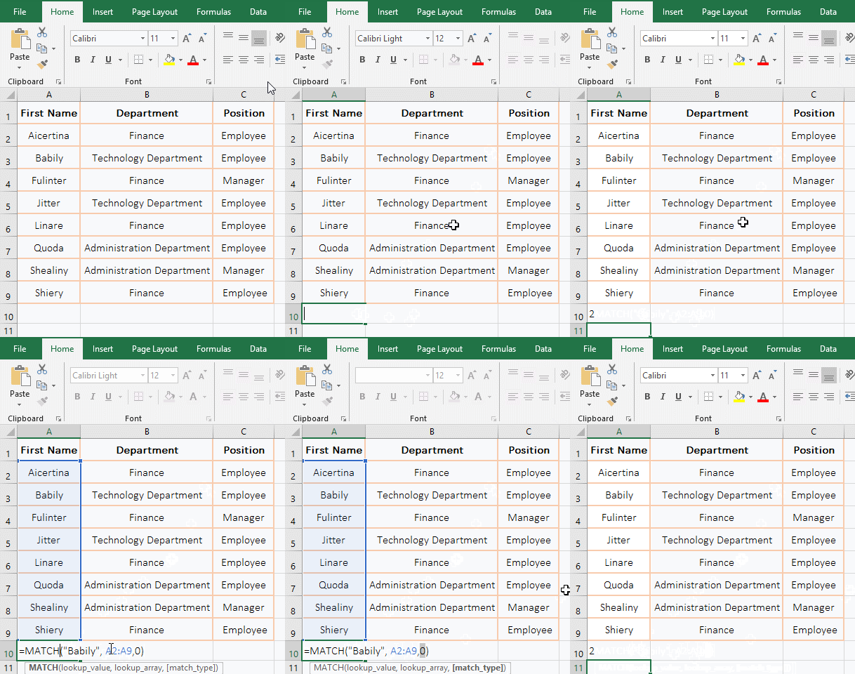
Figure 2
2. Formula description:
A. When the argument Match_Type is 0, when it is not sorted in ascending order, it can still return correctly the position(3) of "Babily" in A2:A9, when Match_Typ is 0, the LookUp_Array is not sorted.
B. Formula =MATCH("Babily", A2:A9,0) and =MATCH("Babily", A2:A9,) can return the same value, indicating that the third argument Match_Type is omitted, if there is a comma(,) after the second argument, and Match_Type takes 0 by default; if there is no comma after the second argument, Match_Type defaults to 1. This should be noted.
(III) Match_Type takes -1
1. If you want to find the sales position of 5500 and 5000 in the fruit sales table. Double-click the cell D8, copy the formula =MATCH(5500,D2:D7,-1) to D8, press Enter to return the error value #N/A; select D8, press the Delete key to delete the formula; select the "Data" tab, click the "Descending" icon(Z→A) to sort the table in descending order by "Sales"; again copy the formula =MATCH(5500,D2:D7,-1) to D8, press Enter, return to position 3 of 5500 in D2:D8; Double-click D8, change 5550 to 5000, press Enter, also return 3; the operation steps are as shown in Figure 3:
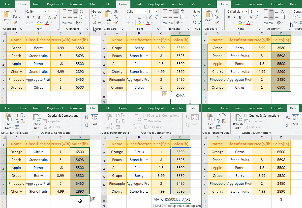
Figure 3
2. Formula description:
A. When Match_Type takes -1, the formula returns the error value #N/A before sorting the "sales" column of the Lookup_Array; When sorted in "descending order", it can return 5500 in the correct position in D2:D8, indicating that Match_Type takes -1, the Lookup_Array must be sorted in descending order; when 5500 is changed to 5000, since there is no 5000 in D2:D8, the minimum value greater than or equal to 5000 is found, that is, 5500, and finally the position of the value is returned.
(IV) Finding a value using wildcard question marks(?) or asterisks(*)
1. If you want to find the position of the fruit name that starts with any four or five characters and ends with "e" in column A. Double-click the cell A8, copy the formula =MATCH("????e",A2:A7,0) to A8, press Enter, return 3; double-click A8, change "????e" to "?????e", press Enter, return 1; double-click A8 again, change "?????e" to "*y", press Enter, return to 6; the operation steps, as shown in Figure 4:
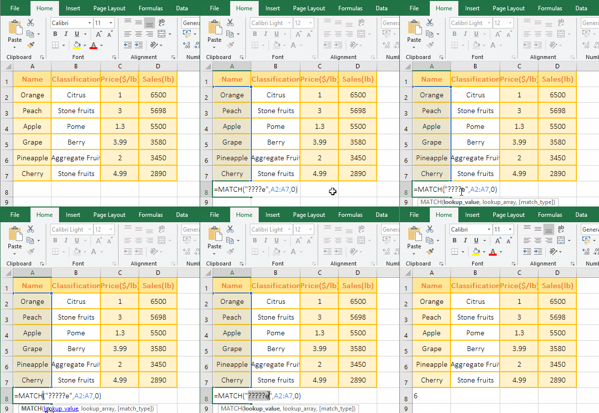
Figure 4
2. Formula description:
The Lookup_Value "????e" in the formula =MATCH("????e",A2:A7,0) has a question mark, it means any four characters, found "Apple", so return to position 3; "?????e" means that it starts with any five characters and ends with "e", so find "Orange"; "*y" means start with any one or more characters and end with "y", so find "Cherry". Using wildcards in addition to the above several ways of searching, you can also combine a variety of search methods, which have been introduced many times in the previous chapter.
III, The expand examples of Excel Match function
(I) Index + Match combination use case
There are two combinations of Index + Match, one is =Index(, Match(,,)), the other is =Index(, Match(,,),Match(,,)). For details, please see the article "How to use excel Index function, include it and Match,Small,If combination achieve multiple criteria and one-to-many lookup".
(II) Indirect + Match combination implementation returns multiple values(extracted data) in the cells at the intersection of rows and columns
1. Double-click cell B10, copy the formula =INDIRECT("r"&MATCH($A10,$A$1:$A$7,)&"c"&COLUMN(),0) to B10, press Enter to return to the "Pome"; select B10, move the mouse to the cell fill handle in the lower right corner of B10, after the mouse turns into a bold black cross, hold down the left button and drag to the right to extract all the data of "Apple"; move the mouse to the cell fill handle in the lower right corner of D10, hold down the left button and drag down to extract all the data of "Cherry". Double click B13, copy the formula =INDEX($A$1:$D$7,MATCH($A13,$A$1:$A$7,),MATCH(B$9,$A$1:$D$1,)) to B13, press Enter, return "Pome", and then drag to the right and drag down to extract the remaining data. The steps are as shown in Figure 5:
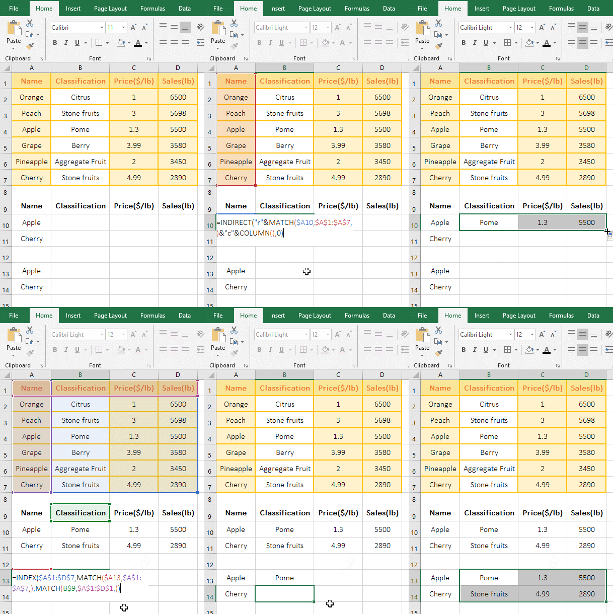
Figure 5
2. Formula description:
(1) Formula =INDIRECT("r"&MATCH($A10,$A$1:$A$7,)&"c"&COLUMN(),0)
A. $A10 means that the absolute reference column and the relative to reference row. When dragging to the right, A10 will not become B10, C10, ...; when dragging down, A10 will become A11, A12, ...; $A$1:$A$7 returns the "Name" in A1:A7 as an array.
B. MATCH($A10, $A$1:$A$7,) is used to return the position of A10(Apple) in A1:A7, the result is 4; COLUMN() is used to return the column number of the cell that contains the formula, when the formula is in B10, return 2.
C. The formula becomes =INDIRECT("r"&4&"c"&2,0), & is the connector, used here to connect the character(or string) with the number, and further calculation becomes =INDIRECT(r4c2,0), r is the row and c is the column in r4c2, r4c2 is the 4th row and the second column, that is, B4; argrment 0 means that the cell reference is interpreted as r1b1; finally, using Indirect function to return a reference to r4c2, that is, returning "Pome" .
(2) Formula =INDEX($A$1:$D$7,MATCH($A13,$A$1:$A$7,),MATCH(B$9,$A$1:$D$1,)) and =INDIRECT(" r"&MATCH($A10,$A$1:$A$7,)&"c"&COLUMN(),0) has the same effect, except that Index + Match refers to the column name of the table in the formula(eg B$9), Indirect + Match does not need to be referenced; for the explanation of Index + Match, please refer to "Index + Match combination example" above.
(III) OffSet + Match combination use example
1. If you want to return the value that corresponds to the minimum value that is greater than and equals the Lookup_Value in a column, for example, look for the "Name" corresponding to the price of 3 or 3.8.
First sort the C columns in "descending order"(the method has been introduced above "(III) Match_Type takes -1"); double-click cell B10, copy the formula =OFFSET(A1,MATCH(A10,C2:C7,-1),) to B10, press Enter, return to "Peach"; double-click C10, copy the formula =VLOOKUP(A10,CHOOSE({1,2},C2:C7,A2:A7),2,) to C10, press Enter , also returns "Peach"; double-click A10, change 3 to 3.8, click B10 (or press Ctrl + S to save), the content of B10 becomes "Grape", the content of C10 becomes the wrong value #N/A; Operation process steps, as shown in Figure 6:
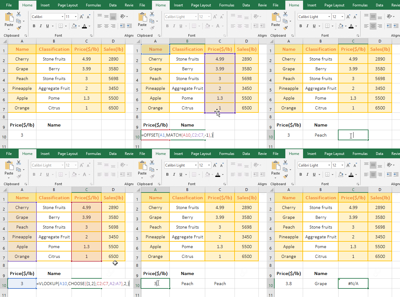
Figure 6
2. Formula =OFFSET(A1,MATCH(A10,C2:C7,-1),) and =VLOOKUP(A10,CHOOSE({1,2},C2:C7,A2:A7),2,) description:
A. MATCH(A10,C2:C7,-1) is used to return the position 3 of A10(3) in C2:C7; the formula change to =OFFSET(A1,3,), then use OffSet function to return the value in the cell where three rows below the a1 and right column 0 of a1, which is exactly the "Peach" in A4.
B. The formula =VLOOKUP(A10,CHOOSE({1,2},C2:C7,A2:A7),2,) and =OFFSET(A1,MATCH(A10,C2:C7,-1),) can return the same value is limited to the Lookup_Value in the LookUp_Array. For example, when A10 is 3, there is 3 in column C; When 3 is changed to 3.8, OffSet + Match can return the correct value, and VLookUp + Choose returns #N/A, indicating OffSet + Match can find a minimum value greater than or equal to the Lookup_Value, while VLookUp + Choose does not. In addition, OffSet + Match is more efficient than VLookUp + Choose.
C. The formula =VLOOKUP(A10,CHOOSE({1,2},C2:C7,A2:A7),2,) has been made the similar introduction in the article "VLookUp in excel introduces step by step(10 examples), include Reverse lookup,one-to-many lookup". If you don't understand it, you can refer to it.
(IV) Excel match multiple criteria: Sum + OffSet + Indirect + Match combination to achieve dynamic cross-table summation of changing ranges
1. If you want to subtotal the sales of women's and men's wear every month, women's sales and men's wear are in a separate table, and they should be subtotaled into the "subtotal" table.
The current worksheet is "Women", click "Men" to switch to the table, click the "Subtotal" worksheet to switch to the table; double-click the B2 cell, copy the formula =SUM(OFFSET(INDIRECT($A2&"!$B$3:$B$7"),,MATCH(B$1,INDIRECT($A2&"!$c$2:$H$2"),))) to B2, Press Enter to return to the "Women's" sales subtotal result of "April" 2480; select B2, use the method of dragging to the right to return the sales subtotal results of the "Women's clothing" remaining months, and then use the method of dragging down to return to the monthly sales subtotal results of "Men's clothing"; the operational process steps, as shown in Figure 7:
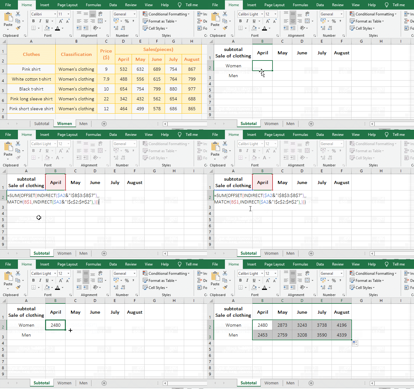
Figure 7
2. Formula =SUM(OFFSET(INDIRECT($A2&"!$B$3:$B$7"),,MATCH(B$1,INDIRECT($A2&"!$c$2:$H$2"),))) description:
A. $A2& returns worksheet names, the value in A2 is "Women". When dragging down, A2 becomes A3, "Women" becomes "Men".
B. $B$3:$B$7 returns the values in B3 to B7 as an array, INDIRECT($A2&"!$B$3:$B$7") turns the character into a reference to the cell. It returns "Women!$B$3:$B$7".
C. $C$2:$H$2 returns the values in C2 to H2 as an array, which returns the column names from C2 to H2; INDIRECT($A2&"!$C$2:$H$2") "Women! $C$2:$H$2".
D. MATCH(B$1,INDIRECT($A2&"!$C$2:$H$2"),) becomes MATCH(B$1,Women!$C$2:$H$2,), Then use Match function to return B1(April) at position 2 in C2 to H2.
E. The formula becomes =SUM(OFFSET(Women!$B$3:$B$7,,2,))), further calculations with OffSet function return "Women!$D3$3:$D$7", is How to return? When executing to OffSet, first take out B3, then return to the cell separated by B3 with two columns, that is, return D3; take out B4 for the second time, return to cell D4 separated from B4 by two columns; the other and so on, so the last return "Women!$D3$3:$D$7"; the formula becomes =SUM(Women!$D$3:$D$7), and finally add the values in D3:D7, so return 2407.
-
Related Reading
- Excel lookup function usage(Multiple conditional and
- Excel SumProduct function(multiple criteria, with if
- VLookUp in excel introduces step by step(10 examples
- How to find duplicate values in excel using vlookup(
- Excel SumIf function with ?/*, Average and array mul
- How to use Excel subtotal function(combine it with O
- How to use excel aggregate function(ignore error val
- How to use hlookup in excel(7 hlookup example, combi
- How to use excel Index function, include it and Matc
- Vlookup with if statement(use if/if{0,1} combination
- Sumifs example step by step in excel(sumifs with tex
- How to sum in excel(9 formulas), include sum use sho