Excel CountA and CountBlank function usage examples(1:1,$A:$A, combine with countif,sum,offset)

The CountA function is used to count the number of cells outside the empty cell in excel. The difference between it and the Count function is that CountA counts the celsl that contain text or logical values, while the Count function does not count. The CountBlank function is dedicated to counting the number of empty cells, including the empty cells returned by the formula.

If you do not count 0 and the formula returns the null cell, you can use the combination of CountA + CountBlank + CountIf; if you want to achieve automatic summation after adding data, you can use the OffSet + CountA function combination; if you want to achieve segmentation statistics, you can use If + Mod + CountA + Row function combination.

I, Excel CountA function and CountBlank function syntax

(I) CountA function

1. Expression: COUNTA(Value1, [Value2], ...)

2. Description:

A. CountA function counts number, date, text, logical values(True and False), null values (such as the null value returned by the formula "") and error values, they can be in cells or arrays; and the Count function only counts number, date and the text that can be converted to a number.

B. The CountA function must have at least one Value, and there can be at most 255 Value.

(II) CountBlank function

1. Expression: COUNTBLANK(Range)

2. Description:

A. CountBlank function counts empty cells, empty text(ie ""), does not count cells with 0.

B. To run the CountBlank function, you need to turn off the iterative calculation, the method: select "File" → Options → Formula → under "Calculation Options" → Uncheck "Enable Iteration Calculation" → OK.

II, The examples of Excel CountA function

(I) Count the cells both existing text and number

1. Double-click thev D8, copy the formula =COUNTA(D1:D7) to D8, press Enter, return to the count result 7; the operation process steps, as shown in Figure 1:

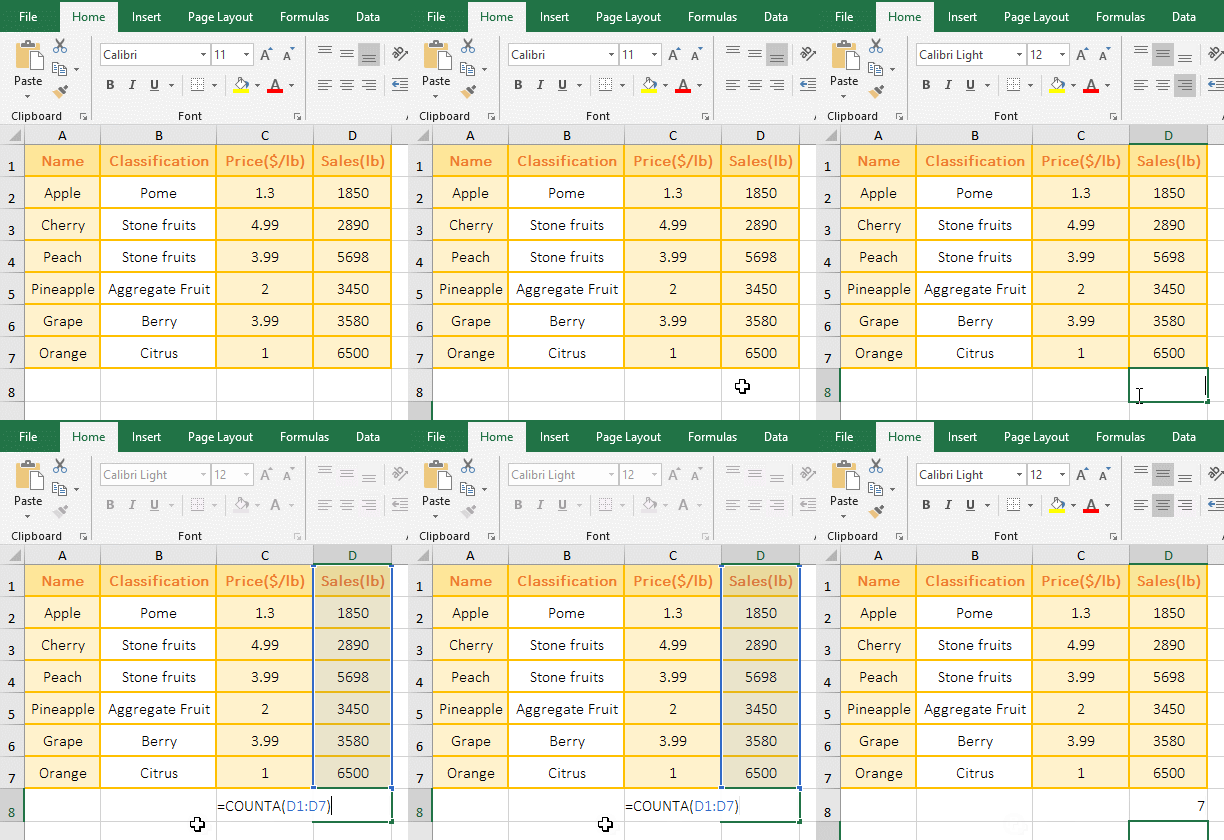
Figure 1

2. There is a cell contain text and 6 cells contain numeric in D1 to D7. The counted result is 7, which indicates the text and numbers are counted.

(II) Count null and error values, empty cells are not counted

1. Double-click the cell A4, copy the formula =COUNTA(A1:A3) to A4, press Enter, return to the counted result 2; double-click A1, there is nothing in the cell; double-click A2, which is an If formula return Empty value; double-click A1, enter 5, the counted result becomes 3; the operation process steps, as shown in Figure 2:

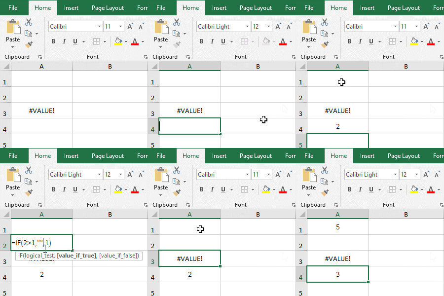
Figure 2

2. When A1 is empty, the counted result is 2. When input 5 in A1, the counted result is 3, indicating that the empty cell is not counted, but the null value returned by the formula is counted.

(III) Count the total number of cells that are not empty in row

1. Count the total number of cells that are not empty in the first row. Double-click the cell A8, copy the formula =COUNTA(1:1) to A8, press Enter, return to the counted result 4; double-click A8 again, add $ before both 1, press Enter, also return 4; operation steps, as shown in Figure 3:

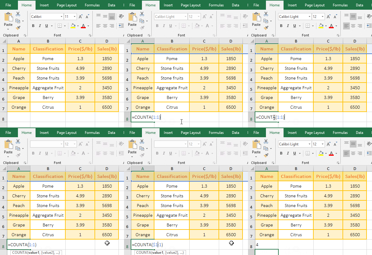
Figure 3

2. Formula description:

The 1:1 in the formula =COUNTA(1:1) representation refers to the first row; the $1:$1 in =COUNTA($1:$1) also refers to the first row, except that 1:1 is a relative reference, and $1:$1 is an absolute reference; if the formula is to be dragged down and you want to drag to the first few rows to count the total number of cells in that row, you should use =COUNTA(1:1), because when dragging down, 1:1 will change For 2:2, 3:3, etc.

Hint: The formulas =COUNTA(1:1) and =COUNTA($1:$1) cannot be written to the first row, otherwise the correct result cannot be counted.

(IV) Count the total number of cells that are not empty in column

1. Count the total number of cells in the first column that are not empty. Double-click the cell B8, copy the formula =COUNTA(A:A) to B8, press Enter, return to the counted result 7; then double-click B8, add $ before both A, press Enter, also return 7; operation steps, as shown in Figure 4:

Figure 4

2. A:A indicates a reference to column A in the formula =COUNTA(A:A), =COUNTA($A:$A) also indicates a reference to column A; A:A and $A:$A are also  the former is relative reference and latter is absolute reference; in addition, the formula cannot be written to column A, otherwise it will return an incorrect value.

(V) Cross-table counts examples

1. If you want to count the total number of cells in B2:B7 in "Frui1 and Fruit2". Currently in the "Fruit1", click the "Fruit2" tab to switch the worksheet, double-click the cell A8, and copy the formula =COUNTA(Fruit1:Fruit2!B2:B7) to A8, press Enter, return to the counted result 12; the process steps, as shown in Figure 5:

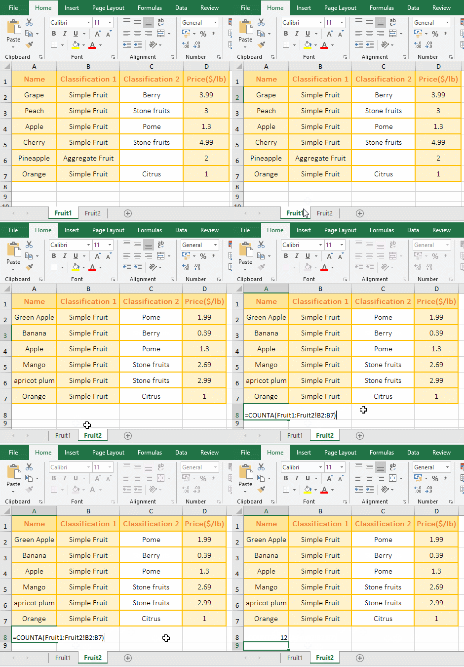
Figure 5

2. Formula description:

"Fruit1:Fruit2" in the formula =COUNTA(Fruit1:Fruit2!B2:B7) indicates that two worksheets are referenced, and ! is used as a separation between worksheets and reference cells. If you refer to two worksheets with the same range, you can write the worksheets together, otherwise you should write the worksheet separately.

III, The examples of Excel CountBlank function

(I) Counted all empty cell

1. Double-click the cell A5, copy the formula =COUNTBLANK(A1:A4) to A5, press Enter, return to the counted result 2; double-click A1, there is an If formula to return the null value "", then double-click A3, it is empty cell; operation process steps, as shown in Figure 6:

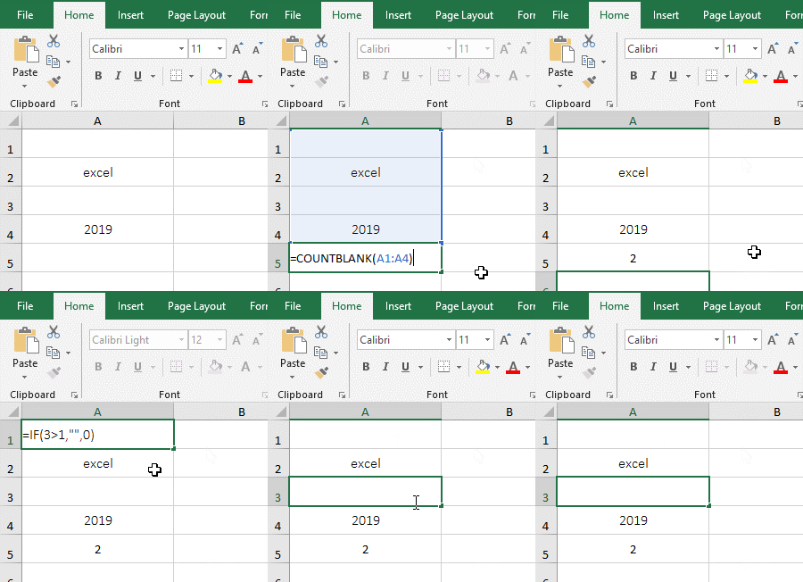
Figure 6

2. There are two empty cells in A1:A4, one is the empty cell returned by the formula, the other is the empty cell without any text, both are counted, indicating that the CountBlank function counts them.

(II) CountBlank, Countif and CountA function combination does not count 0 and the formula returns a null value

1. Double-click the cell A5, copy the formula =COUNTA(A1:A4)-COUNTBLANK(A1:A4)-COUNTIF(A1:A4,"=0") to A5, press Enter to return to the counted result 2; double-click A1, there is an If formula that returns a null value "" in the cell; the operation steps are as shown in Figure 7:

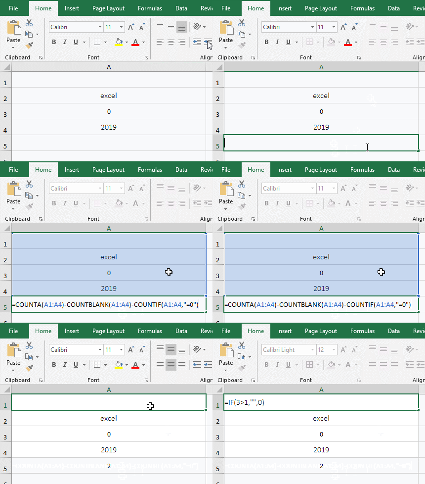
Figure 7

2. Formula =COUNTA(A1:A4)-COUNTBLANK(A1:A4)-COUNTIF(A1:A4,"=0") explanation:

=COUNTA(A1:A4) is used to count the number of text, values, and empty cell in A1:A4, and the result is 4; COUNTBLANK(A1:A4) is used to count the number of empty cell in A1:A4, the result is 1; COUNTIF(A1:A4,"=0") is used to count the number of 0 in A1:A4, and the result is 1; the counted results of each part are subtracted, that is, 4 - 1 - 1, so the final result is 2.

IV, Excel CountA function extension use case

(I) OffSet + CountA function combination to achieve automatic summation after adding data

1. If you want to achieve automatic summation after adding sales in the last row in the table. Double-click the cell E2, copy the formula =SUM(OFFSET(D1,1,,COUNTA(D:D)-1)) to E2, press Enter, return to the summation result 23968; double-click D8, enter 5689, press Enter the value in E2 automatically changes to 29657, indicating that the new input 5689 is added; the operation steps are as shown in Figure 8:

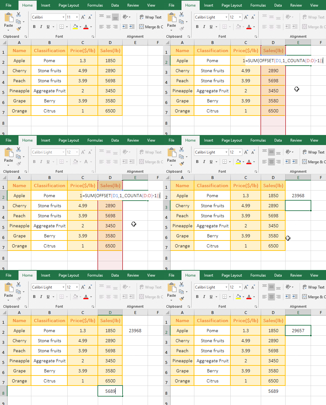
Figure 8

2. The formula =SUM(OFFSET(D1,1,,COUNTA(D:D)-1)) description:

A. COUNTA (D:D) is used to count the total number of cells with content in column D, the result is 7, which is exactly the total number of cells in D1:D7; then subtract 7 from 1, and the result is 6.

B. OFFSET(D1,1,,COUNTA(D:D)-1) becomes OFFSET(D1,1,,6), and then returns to the reference to cells 1 row under D1 and 0 column to right of D1 and height to 6,that is, the reference to D2:D7.

C. The formula becomes =SUM(D2:D7), and finally adds each number in D2:D7, and the final result is 29657. When 5689 is entered in the last row D8, the counted result of COUNTA(D:D) becomes 8, 8 minus 1 and becomes 7, then OffSet returns D2:D8, so every time a row is added after the table, the formula will automatically add it.

(II) If + Mod + CountA + Row function combination to achieve segmentation statistics

1. If you want to count the number of sales in May and June. Double-click on the cell E2, copy the formula =IF(MOD(ROW()-2,4)=0, COUNTA(OFFSET($D$2:$D$5,INT((ROW()-2)/4)*4, )),"") to E2, press Enter, return to counted 3; select E2, move the mouse to the lower right corner of E2, press the left button after the mouse becomes the bold black plus, drag down until the last row, respectively, the number of sales of "May and June" is counted, and the operation steps are as shown in Figure 9:

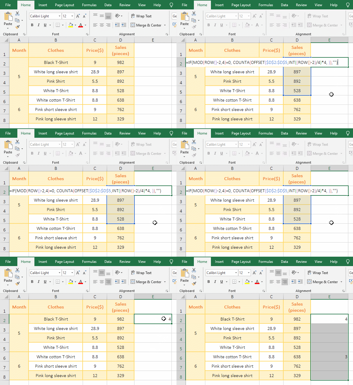
Figure 9

2. Formula =IF(MOD(ROW()-2,4)=0, COUNTA(OFFSET($D$2:$D$5,INT((ROW()-2)/4)*4, )),"") description:

A, 4 in the formula means that one segment is four rows, ROW() returns the row number 2 of cell where the formula is located, then (ROW()-2)/4 returns 0; the Int function is used for rounding, then INT(0) returns 0.

B. Then OFFSET($D$2:$D$5,INT((ROW()-2)/4)*4,) becomes OFFSET($D$2:$D$5,0*4,), then use OffSet function returns the reference to cells 0 row under D2 and 0 coulumn to right of D2 and the same height and width as D2:D5, which returns D2:D5.

C. Then COUNTA(OFFSET($D$2:$D$5, INT((ROW()-2)/4)*4,)) becomes COUNTA($D$2:$D$5), further calculation, for D2:D5 is counted and the result is 3.

D. The formula becomes =IF(MOD(ROW()-2,4)=0,3,""); since ROW() returns 2, MOD(ROW()-2,4) becomes MOD(2-2, 4), then use Mod function to modulo 0 and 4, the result is 0; then the formula becomes =IF(0=0,3,""), since the condition 0=0 of if function is established, it returns 3.

E. When the formula is at E6, ROW() returns 6 and substitutes INT((ROW()-2)/4) for INT((6-2)/4). Further calculation becomes INT(1), and the result is 1; then OFFSET($D$2:$D$5,INT((ROW()-2)/4)*4,) becomes OFFSET($D$2:$D$5,1*4,), and then returns the reference to cells 4 rows under D2 and 0 coulumn to right of D2 and the same height and width as D2:D5, which returns D6:D9. The following calculation method is the same as above.