How to use Replace function in excel(9 examples, with character and text in formula)

Both the Replace and ReplaceB function are used to replace a specified number of characters with a specified character from a specific position in Excel; but the two functions differ: when replaced, the Replace function counts a half-width characters(such as "number and letter") and the full-width characters(such as "Chinese, Japanese characters and Korean characters") as one character; the ReplaceB function is counted in bytes, which counts half-width characters as one byte and the full-width characters as two bytes,  when you have enabled the editing of a language that supports DBCS and then set it as the default language. In addition, the Substitute function is similar to the Replace function, it replaces another character with one character, there is no replacement from the first digit.

The Replace and ReplaceB function are often used in combination with the Find, Left, Upper, Lower, and Rept functions. For example, the Replace + Find + Rept combination is implemented from any specified character to the end, and the Replace + Find + Find combination replaces the string between any two characters, the Replace + Upper + Left combination capitalizes the first letter of the sentence.

I, Excel Replace function and ReplaceB function syntax

1. Replace function expression: REPLACE(Old_Text, Start_Num, Num_Chars, New_Text)

2. ReplaceB function expression: REPLACEB(Old_Text, Start_Num, Num_Bytes, New_Text)

3. Description:

Both the Replace and ReplaceB function are used to replace a specified number of characters from the specified position, but they differ: when replacing characters, the Replace function is in characters, which counts full-width(such as "Chinese, Japanese characters and Korean characters") and half-width (such as "numbers and letters") characters as 1 character; the ReplaceB function is counted in bytes, which counts full-width characters as 2 bytes and half-width characters as 1 byte.

II, How to use Replace function in excel

(I) Excel replace character in string

1. If you want to replace a string of letters and numbers in the "White 965grf609 cotton T-Shirt". Double-click the cell B1, copy the formula =REPLACE(A1,7,10,"") to B1, press Enter, and return to the "White cotton T-Shirt"; the operation steps are as shown in Figure 1:

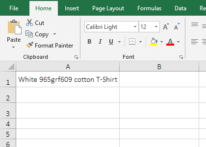
Figure 1

2. Formula description:

In formula =REPLACE(A1,7,10,""), A1 is the Old_Tex, 7 is the Start_Num, 10 is the Num_Chars,

2. Formula description:

In formula =REPLACE(A1,7,10,""), A1 is the Old_Tex, 7 is the Start_Num, 10 is the Num_Chars, and the empty text "" is the New_Text, the meaning of the formula: Replace 965grf609 in A1 with "".

(II) Examples of replacing special characters(Excel formula to replace characters in a cell)

1. If you want to replace "*/?" in "Excel */? tutolail" with "function". Double-click the cell B1, copy the formula =REPLACE(A1,7,3,"function") to B1, press Enter, return to "Excel function tutorial"; the operation steps are as shown in Figure 2:

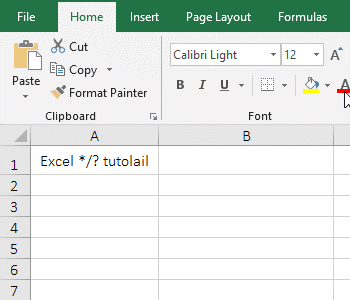
Figure 2

2. Formula description:

Formula =REPLACE(A1,7,3,"function") means to replace 3 characters from the 7th character of A1's text and replace it with the word "function", ie 3 characters are replaced with "function".

(III) Excel replace last character: Replace 4 digits after a number(such as "mobile number") with *

1. Double-click the cell B1, copy the formula =REPLACE(A1,8,4,"****") to B1, press Enter, return to "1696391****"; select B1, move the mouse to the cell fill handle in the lower right corner of B1, after the mouse becomes the bold black plus, double-click the left button, then the last four digits of the remaining mobile numbers are also replaced by *; the operation steps are as shown in Figure 3:

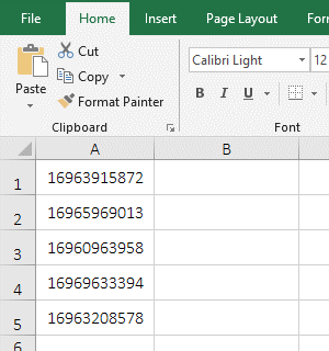
Figure 3

2. Formula description:

The formula =REPLACE(A1,8,4,"****") means that the number in A1 is replaced with **** from the 8th digit and only 4 digits are replaced.

(IV) Replace all character after any specified character(How to replace text in excel)

1. If you want to replace all the characters after "tutorial" in "Excel tutolail1dg9sh9gfd863rt91g788d587gf2kd0f2". Double-click the cell B1, copy the formula =REPLACE(A1,15,32699,"") to B1, press Enter, return to "Excel tutorial"; the operation steps are as shown in Figure 4:

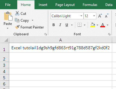
Figure 4

2. Formula description:

32699 is the maximum number of characters allowed by the Replace function in formula =REPLACE(A1,15,32699,""). The formula means: Replace 32699 characters with "" from the 8th bit of text in A1(that is, from the first character after the "tutolail").

III, How to use ReplaceB function in excel

(I) Examples of replacing numbers and letters

1. If you want to replace "gk963" in "890675gk963" with 0. Double-click the cell B1, copy the formula =REPLACEB(A1,7,5,"00000") to B1, press Enter, return to 89067500000; the operation steps are as shown in Figure 5:

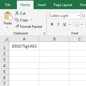
Figure 5

2. Formula description:

A1 is the Old_Text, 7 is the Start_Num, 5 is the Num_Bytes, 00000 is the New_Text in formula =REPLACEB(A1,7,5,"00000"), the meaning of the formula: Replace 5 characters with 00000 from the 7th character in A1.

IV, The application example of Excel Replace and ReplaceB function

(I) Replace + Find + Rept function combination replaces from any specified character

1. If you want to replace the numbers after "k" in A column with 0. Double-click the cell B1, copy the formula =REPLACE(A1,FIND("k",A1),32699,REPT("0",3)) to B1, press Enter to return to 890675000; select B1, Replaces the remaining the contents in cells with the method of double-click the cell fill handle; the operation steps are as shown in Figure 6:

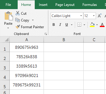
Figure 6

2. Formula =REPLACE(A1,FIND("k",A1),32699,REPT("0",3)) description:

A. FIND("k",A1) is used to return the position of the letter "k" in A1, the result is 7; the Find function counts both full-width and half-width characters as one character.

B. REPT("0",3) is used to repeat 0 3 times, the result is 000. the role of the Rept function is to repeat any specified character a specified number of times, often used when a character or phrase is repeated multiple times.

C. The formula becomes =REPLACE(A1,7,32699,"000"), and finally replaces 32699 characters with 000 from the 7th character in A1, 32699 has been explained above.

In addition, the same function can be achieved with ReplaceB + FindB + Rept. The formula can be written like this: =REPLACEB(A1,FINDB("k",A1),32699,REPT("0",3)), it is worth noting that: the full-width characters occupies 2 bytes.

(II) Replace + Find + Find function combination replaces the string between any two characters

1. If you want to replace the string in the bracket [] and bracket in the text "890675[k963*kj3u3tirt4u0gj7G]697896". Double-click the cell B2, copy the formula =REPLACE(A1,FIND("[",A1),FIND("]",A1)-FIND("[",A1)+1,"") to A2, press Enter, returns the text that was replaced; the operational steps are as shown in Figure 7:

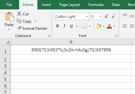
Figure 7

2. Formula =REPLACE(A1,FIND("[",A1),FIND("]",A1)-FIND("[",A1)+1,"") description:

A. FIND("[",A1) returns the position of left bracket [ in A1, the result is 7; FIND("]",A1) returns the position of right bracket ] in A1, the result is 29.

B. FIND("]",A1)-FIND("[",A1)+1 calculate the length of the string to be intercepted, use the position of the next bracket ] minus the position of the previous bracket [and add 1, ie 29 - 7 + 1, the result is 23, which is exactly the number of characters from the left bracket [ to the right bracket ], and contains two brackets.

C. The formula becomes =REPLACE(A1,7,23,""), and finally replaces 23 characters with "" from the 7th character of A1.

(III) Upgrade the phone number with the Replace function.

1. If you want to upgrade your phone number from 7 to 8 digits. Double-click the cell B2, copy the formula =REPLACE(A2,8,1,3) to B2, press Enter, return to the upgraded 1-digit phone number; double-click the cell fill handle of B2 to upgrade the remaining number; the steps are as shown in Figure 8:

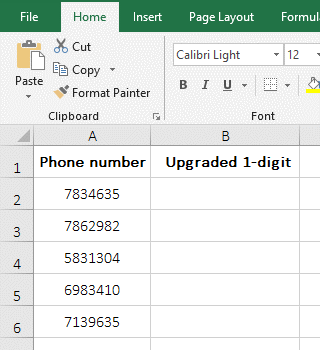
Figure 8

2. Formula =REPLACE(A2,8,1,3) description:

The phone number in A2 is only 7 digits, but the formula =REPLACE(A2,8,1,3) can be replaced from the 8th digit. Just replace 1 digit, then the phone number is upgraded to 8 digits; if you want to batch generate, the last 1 bit can only be replaced with the same number.

(IV) Replace + Upper + Left function combination to achieve initial capitalization

1. If you want to capitalize the first letter of the sentence in column A. Double-click the cell B2, copy the formula =REPLACE(A2,1,1,UPPER(LEFT(A2,1))) to B2, press Enter, and return to the sentence in A2 from lowercase to uppercase; capitalize the initial by double-clicking the cell fill handle; the operation steps are as shown in Figure 9:

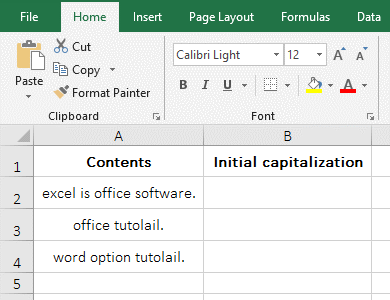
Figure 9

2. Formula =REPLACE(A2,1,1,UPPER(LEFT(A2,1))) description:

A. LEFT(A2,1) is used to intercept 1 letter from the first digit on the left side of sentence in A2, and the result is "e". The Upper function is used to convert lowercase letters to uppercase letters, and UPPER(e) returns E.

B. The formula becomes =REPLACE(A2,1,1,"E"), and finally replace 1 letter of the sentence in A2 with "E" from the first digit, then the lowercase "e" is replaced with the uppercase "E", also capitalize the first letter of the sentence.