How to freeze panes in excel and split window(15 example, with top row or column, unfreeze and vba)

The freeze panes can either freeze the first row or column and freeze any ofthe first few rows or columns in Excel. It can also freeze the first row and first column, any of the first few rows and columns at once. The split window can split a table into two windows, and split it into four windows, which have the same effect as the freeze panes.

If you want to dynamically freeze and bulk freeze the panes, you need to use VBA(macro) to achieve. For example, VBA can be used to freeze any arbitrarily designated cells or selected cells from a worksheet, multiple worksheets or all worksheets of a workbook. It is also possible to freeze only all selected worksheets.

I, How to freeze panes in excel

(1) How to freeze top row in excel(How to freeze first row in excel)

Select the "View" tab, click "Freeze Panes", select "Freeze Top Row" in the pop-up menu, a gray line appears on the lower line of the first row, then the first row is frozen, when dragging the slider down, the data is move up, the first row always stops at the first row; the operation steps are as shown in Figure 1:

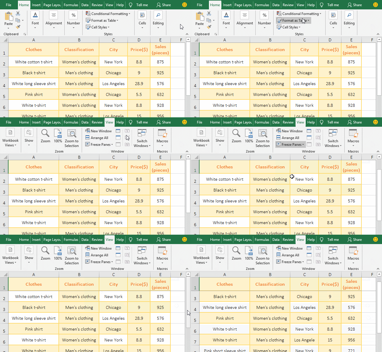
Figure 1

(2) How to freeze first column in excel

The current tab is "View", click "Freeze Panes", select "Freeze First Column" in the pop-up options, a gray line appears on the right line of the first column, then the first column is frozen, when dragging the slider to the right, the column is moved to the left, the first column always stops in the first column; the operation steps are as shown in Figure 2:

Figure 2

(3) Excel freeze top row and first column at the same time

The current tab is "View", select the cell B2, click "Freeze Panes", select "Freeze Panes" in the pop-up menu, then a gray line appears on the right line of column A and the lower line of the first row respectively, the top row and the first column are frozen at the same time; when moving the data upwards, the first row does not move; when moving the data to the left, the first column does not move; the operation steps are as shown in Figure 3:

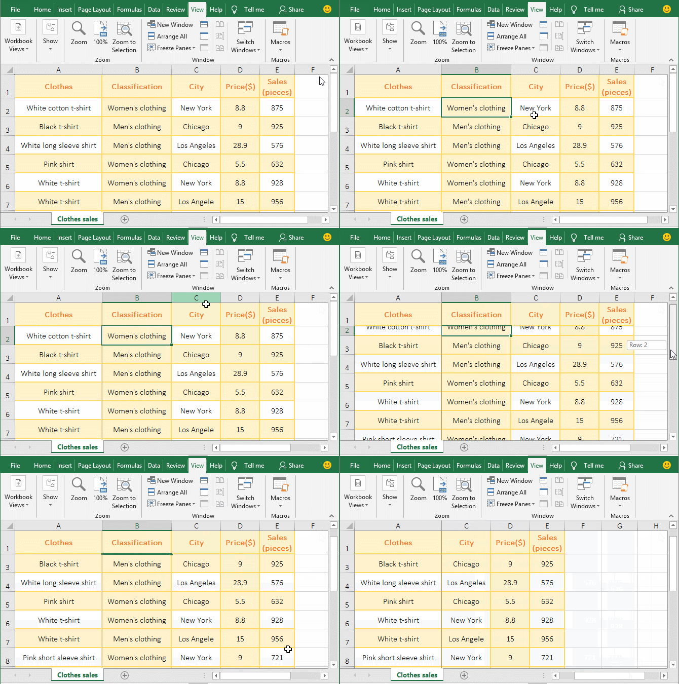
Figure 3

(4) How to freeze multiple rows in excel(eg. How to freeze first two rows in excel)

Select the cell A3, click "Freeze Panes" under the "View" tab, and then select "Freeze Panes", then a gray line appears on the lower line of the second line, the first tow rows are frozen; when moving the data up, the first two rows don't move; the operation process steps are as shown in Figure 4:

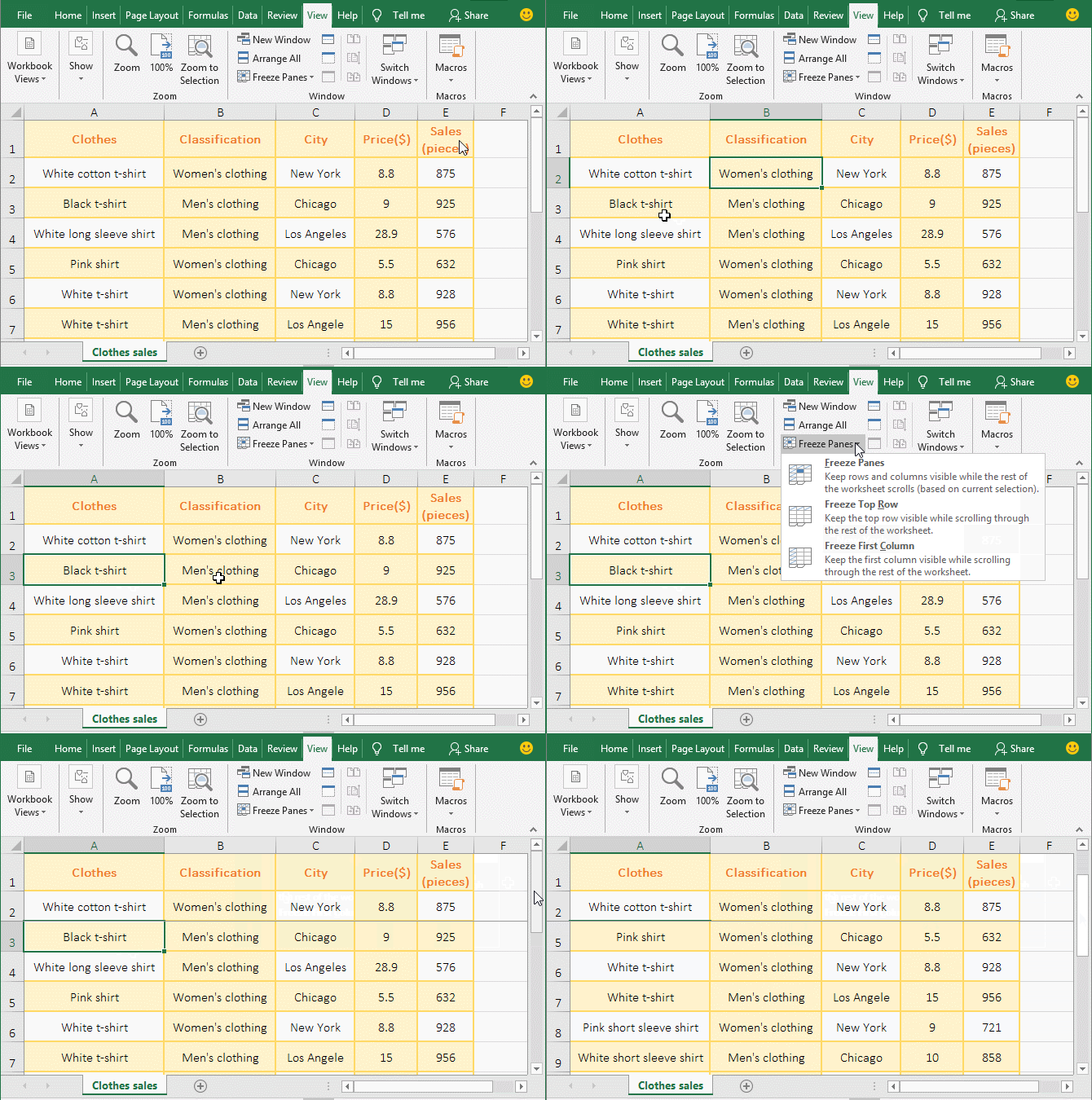
Figure 4

(5) How to freeze multiple columns in excel(eg. How to freeze first two columns in excel)

Select the cell C1, select the "View" tab, click "Freeze Panes", and then select "Freeze Panes" in the pop-up menu, then a gray line appears on the right line of the second column, the first two columns are frozen; when moving data to the left, the first two columns don't move; the operation process steps are as shown in Figure 5:

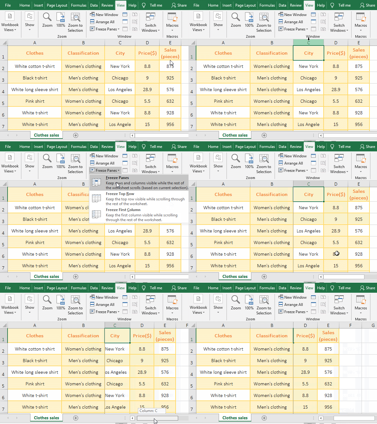
Figure 5

(6) How to freeze columns and rows in excel

If you want to freeze the first 4 rows and the first two columns. Select the cell C5, click "Freeze Panes" under the "View" tab, and then select "Freeze Panes", then a gray line appears in the right line of the B column and the lower line of the fourth row, the first 4 rows and the first two columns both are frozen; when moving data up, the first 4 rows don't move; when moving data to the left, the first two columns don't move; the operation steps are as shown in Figure 6:

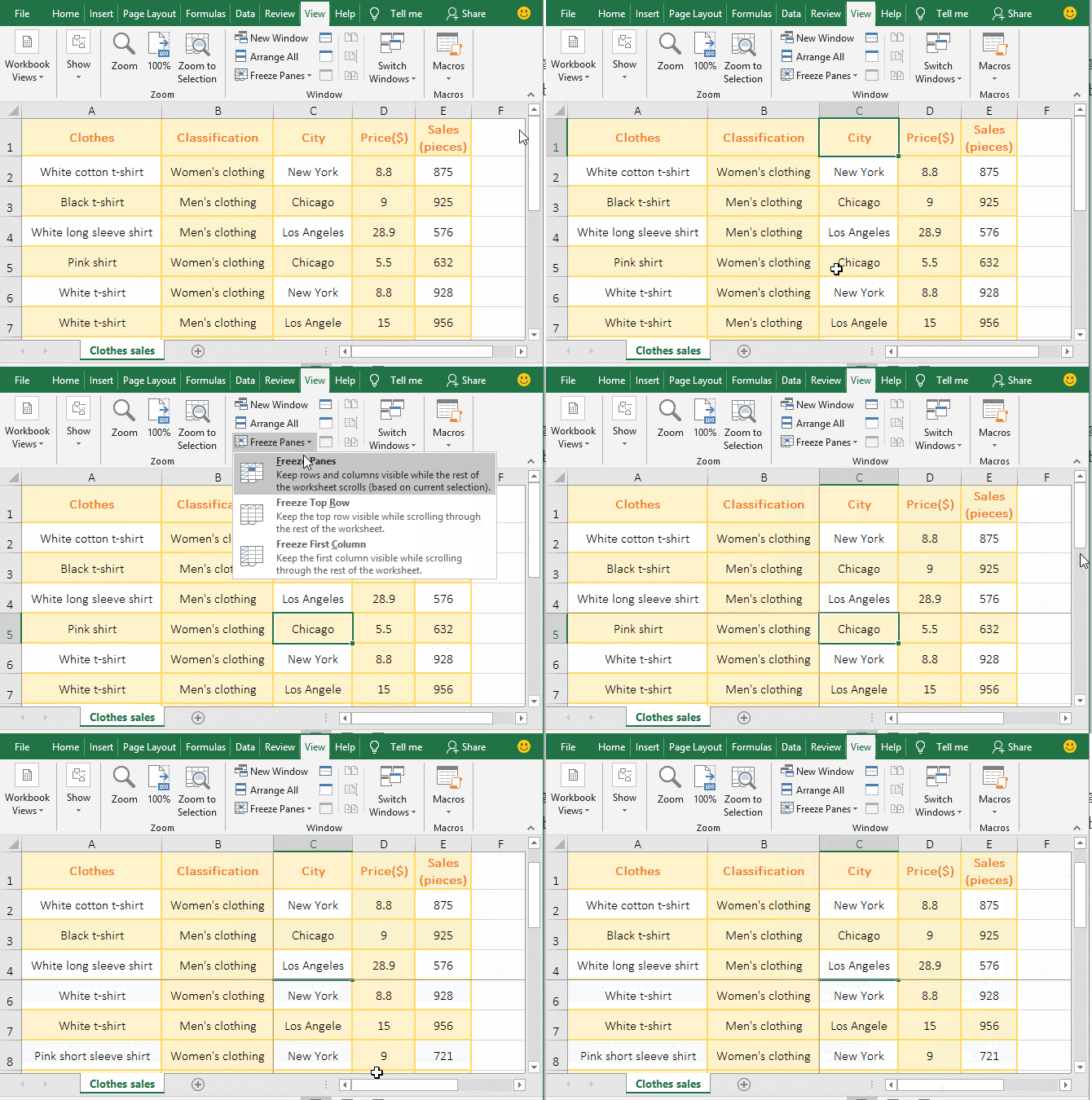
Figure 6

(7) How to unfreeze panes in excel

1. Select the "View" tab, click "Freeze Panes", select "Unfreeze Panes" in the pop-up menu, the first two columns of freezing are Unfreezed. Other freezes are the same unfreezed method; the operation steps are as shown in Figure 7:

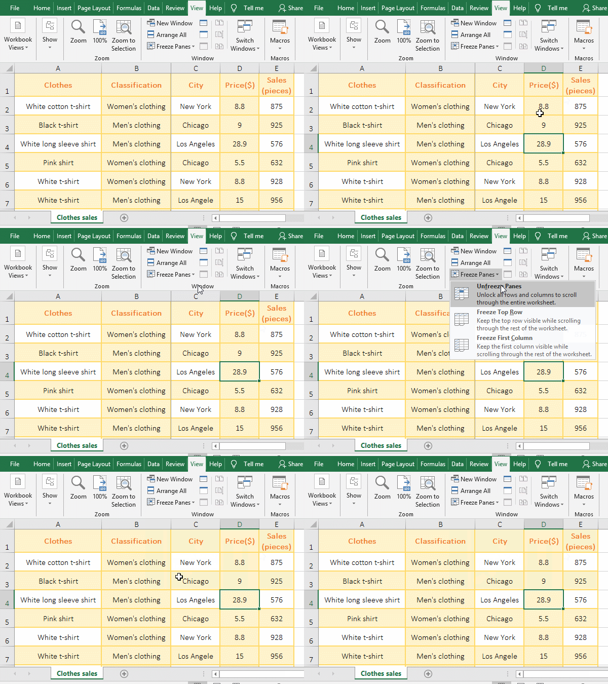
Figure 7

2. Tips:

A. If you select a freeze method(such as "freeze first row") and then choose another freeze method(such as "freeze the first few rows"), the previous freeze method(such as "freeze first row") is canceled.

B. In addition, if it is frozen, the "View" tab is grayed out and it cannot be unfreezed, check whether the worksheet is protected.(Method: select "Review" tab, click "Protect Sheet" or "Protect Workbook",they are in "Tools → Protect" in Excel2003, if a password is required, protection is set). If protection is set, cancel the protection and cancel the freeze.

II, Excel freeze panes shortcut operation

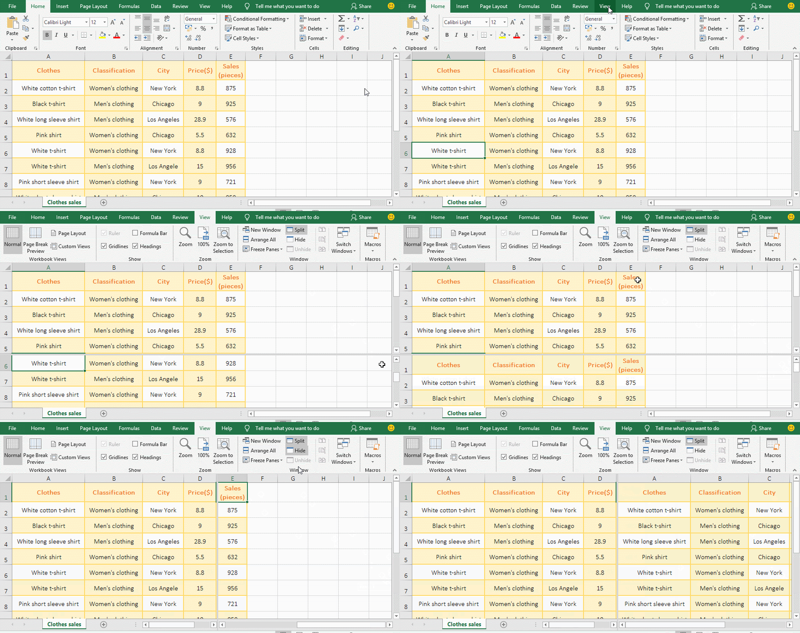
1. Freeze the first row with shortcut. Hold Alt, press W, F, and R one by one, and a gray line appears on the lower line of the first row, drag the slider down, the data is moved up, the first row does not move, indicating that it is frozen; Operation process steps, see screenshot in Figure 8:

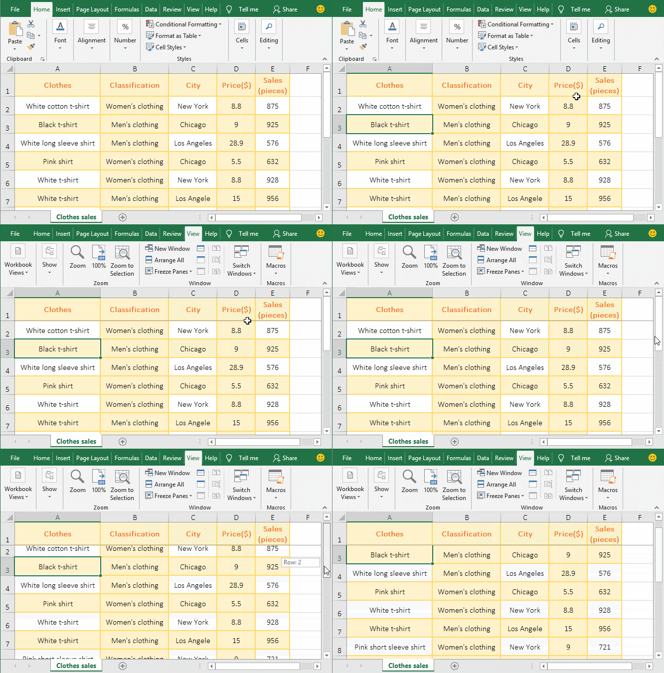
Figure 8

2. The shortcut keys for freezing the first column is Alt + W + F + C. The key press method is: hold down Alt and press W, F and C in sequence.

3. How to freeze rows and columns in excel shortcut key(eg. Freeze the first 5 rows and first 3 columns at a time)

Selectcell D6 , hold down Alt, press W once, press F twice, then a gray line will appear on the lower line of the fifth row and the right line of the third line; when moving the data up, the first five rows will not move; When moving data to the left, the first three columns don't move; the first five rows and the first three columns are frozen; the operation steps are as shown in Figure 9:

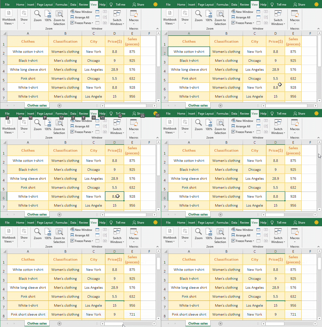
Figure 9

III, Excel split window

(1) How to split excel into 2 windows

1. If you want to split into two windows from the 6th row or 5th column. Select the cell A6, select the "View" tab, click "Split", then split into the second window from the sixth row, drag the slider of the second window up, the window also shows Header row; click "Split" again and the window split is canceled.

2. Select the cell E1 and click "Split" to split it into the second window from the E column. When you move the slider of the second window to the left, the second window is also displayed the same data as the first window; the operation process steps, see screenshot in Figure 10:

Figure 10

(2) How to split into four windows

Select the cell E5, select the "View" tab, click "Split", then split the table from E5 into four windows with the same data; the process steps, see screenshot in Figure 11:

Figure 11

(3) Cancel the split window

Select the "View" tab,  click on "Split"again, the split window is cancelled, Figure 10 has been demonstrated. Freeze rows or column and split windows have the same effect, but they can only be used one at a time. If you have used frozen rows or columns, and then use split windows, the frozen rows or columns are automatically canceled; vice versa.

IV, Excel vba freeze panes

(1) Freeze from any specified cell

1. If you want to freeze from the cell B4. In the Excel window, press Alt + F11, switch to the VBA window, click "Insert", select "Module" in the pop-up menu, create a new module window, copy the following code to the window:

Sub FreezeWindow()
ActiveWindow.FreezePanes = False
Range("B4").Select
ActiveWindow.FreezePanes = True
End Sub

Click "Run", select "Run Sub/User Form" in the pop-up menu, then freeze the first three rows and A column at B4, press Alt + F11, switch back to Excel window, two gray lines intersecting at the upper left corner of B4 have appeared; the operational steps, see screenshot in Figure 12:

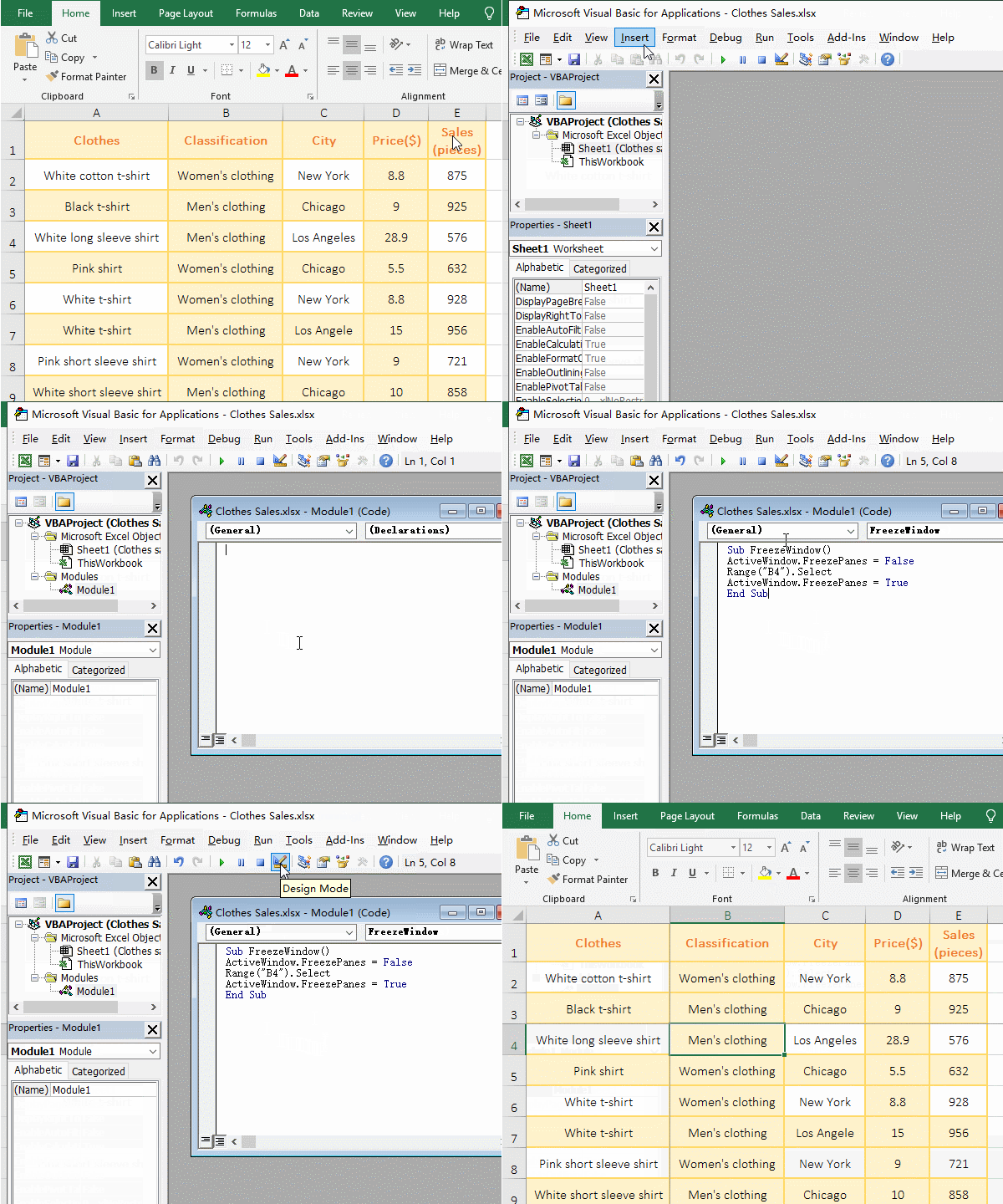
Figure 12

Tip: If you want to freeze in another cell(such as C8), just change B4 in the code to C8.

2. The code description:

A. The "Sub" denotes a Subroutine(function), "FreezeWindow" is the name of the Subroutine, and the "End Sub" denotes the end of the Subroutine.

B. "ActiveWindow" represents the active window, here represents Sheet1; "FreezePanes" means freeze; ActiveWindow.FreezePanes = False Set ActiveWindow.FreezePanes to False, which means that Sheet1 is not frozen.

C. The Range("B4").Select means that cell B4 is selected, Range("B4") means B4 cell is referenced, and the "Select" means selection.

D. The "ActiveWindow.FreezePanes = True" Set ActiveWindow.FreezePanes to True, means to freeze Sheet1, which is frozen from the upper left corner of the B4 cell.

(2) Unfreeze

In the Excel window, press Alt + F11, switch to the VBA window and put the following code:

Sub CancelFreezeWindow()
ActiveWindow.FreezePanes = False
End Sub

Copy to the window "Clothe Sales.xlsx - Module1(Code)"(if there is no such window, click "Insert", select "Module" to create), press F5 to run the code, then press Alt + F11 to switch back to Excel window, the two gray lines in the upper left corner of the cell B4 are no gone, indicating that the freeze was canceled; the operation steps are as shown in Figure 13:

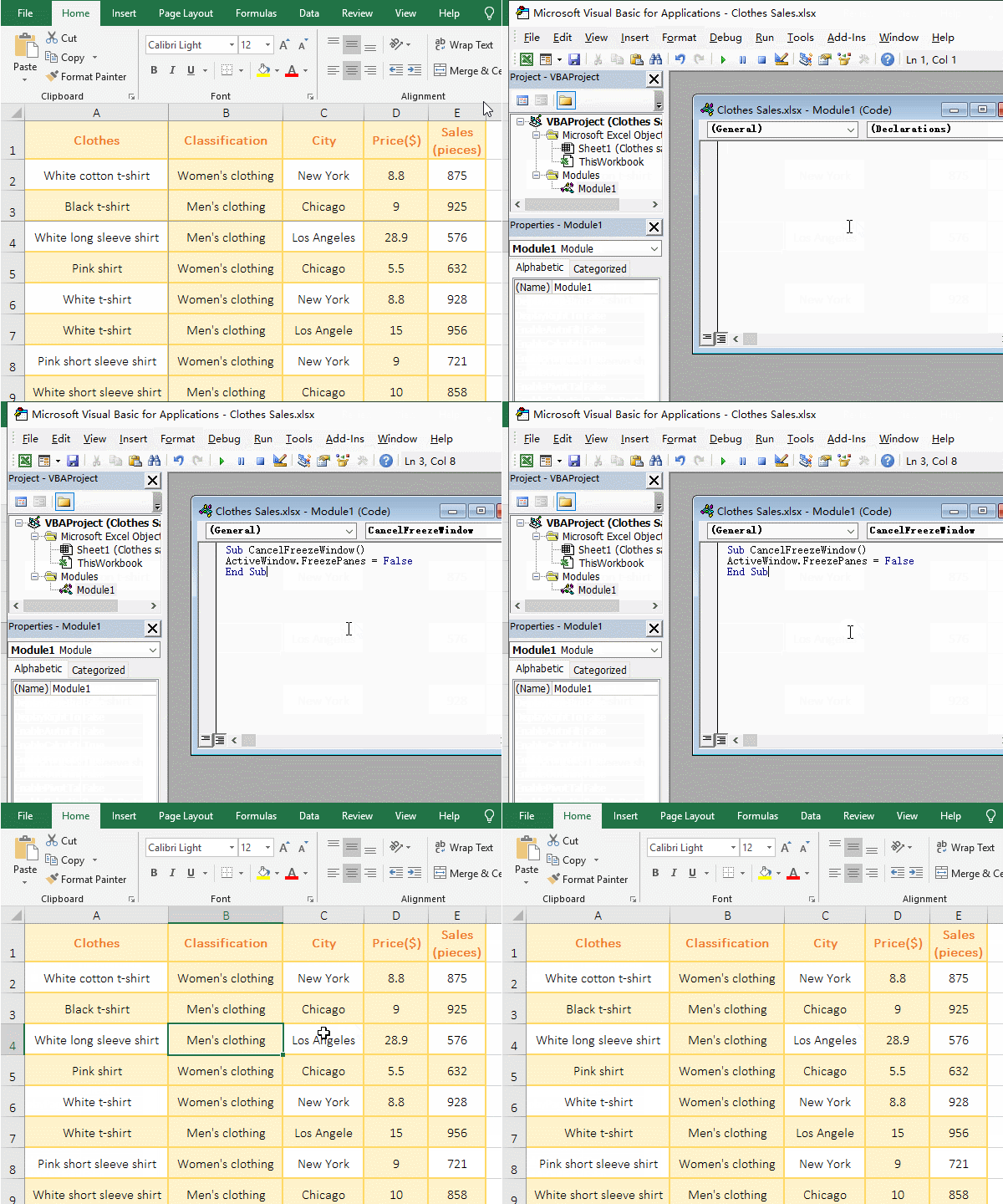
Figure 13

(3) Freeze window and unfreeze in batches

1. Freeze all worksheets from any specified cell in batches

A. If you want to freeze panes from B4(B4 can be arbitrarily replaced with other cells). In the Excel window, press Alt + F11, switch to the VBA window, click "Insert", select "Module" in the pop-up options, create a new module window, and put the following code:

Sub FreezeWindows()
Dim ws As Worksheet
Application.ScreenUpdating = False
For Each ws In ActiveWorkbook.Worksheets
  ws.Activate
  Range("B4").Select
  ActiveWindow.FreezePanes = Not ActiveWindow.FreezePanes
Next
Application.ScreenUpdating = True
End Sub

Copy to this window, press F5 to run the code, press Alt + F11 to switch to the Excel window, the threes sheets "April,May and June" are frozen at B4; press Alt + F11 to switch to the VBA window, then press F5 to run code again, then switch back to the Excel window, the freeze panes of all worksheets are canceled; the operation process steps, as shown in Figure 14:

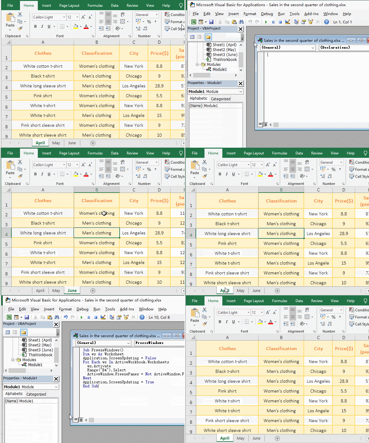
Figure 14

Tip: If you want to freeze the panes at the currently selected cell of each worksheet, do not use Range("B4").Select.

B. Code description:

(1) The "Dim ws As Worksheet" means to define "ws" as a Worksheet object, which is defined as a worksheet.

(2) Application.ScreenUpdating is used to set whether to allow screen refresh, set to False not allowed, set to True to allow.

(3) The "For Each ...Next" is a loop statement; the "ActiveWorkbook" represents the current workbook, the "Worksheets" represents all the worksheets of the current workbook; the "For Each ws In ActiveWorkbook.Worksheets" means to traverse each worksheet of the current workbook one by one, and the "ws" represents the current worksheet; for example, first, "ws" represents Sheet1, second, "ws" represents sheet2, and so on.

(4) The ws.Activate means to set the worksheet as the active worksheet(ie the current worksheet).

(5) Thw Range("B4").Select means to select the cell B4 in the current worksheet, and the Range function is used to reference the cell.

(6) The ActiveWindow.FreezePanes indicates whether the active window(ie the current window) is set to freeze, set it to True, then freeze; set it to False, it does not freeze; set it to "Not ActiveWindow.FreezePanes", which means taking the opposite value of ActiveWindow.FreezePanes; if True is the value of ActiveWindow.FreezePanes, its value is False; if False is the value of ActiveWindow.FreezePanes, its value is True.

2. Only freeze the selected worksheets

A. Take the freeze at the cell B4 in all selected worksheets as an example. In the Excel window, the current worksheet is "April", hold down Shift, click the "May", select both "April and May"; press Alt + F11 to switch to the VBA  window, click "Insert", select "Module", and create a new module window, put the following code:

Sub FreezeWindows()
Dim selWs As Worksheet
  For Each selWs In ActiveWindow.SelectedSheets
    selWs.Activate
    Range("B4").Select
    ActiveWindow.FreezePanes = Not ActiveWindow.FreezePanes
  Next
End Sub

Copy to the module window, press F5 to run, press Alt + F11, switch back to the Excel window, "April and May" are frozen, and "June" is not frozen; the operation steps are as shown in Figure 15:

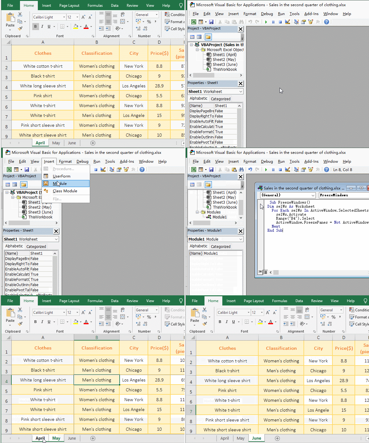
Figure 15

Tip: If you want to freeze from the selected cell of each selected worksheet, remove Range("B4").Select.

B. Code description:

The code is basically the same as the previous example. Just change the traversal of all the worksheets to traverse the selected worksheet, that is, change the "For Each ws In ActiveWorkbook.Worksheets" to "For Each selWs In ActiveWindow.SelectedSheets", the "SelectedSheets" represent all selected worksheets.