 Office > Excel > Excel 2019 > Content
How to use Excel Text function(18 examples, with text, date, condition and {0,1}/{1,-1} format)
The Text function is used to convert a value or date to text by a specified format in Excel. When converting a value to text, you can keep the decimal or round, add the thousands separator, currency symbol and percent sign, you can also use the scientific notation to represent the value; when converting the date and time to text, you can define the year, month, day, hour, minute, and second to display a few digits, or use the corresponding word or its abbreviation.
You can take conditions in the format of the Text function, and you can take one condition and multiple conditions. In addition, arrays can be used in both Value and Format_Text arguments, such as {0,1}, {1,-1}, {-1,1}, etc. in Value, which is often used in conjunction with the Value and VlookUp functions to lookup the specify value.
I, The syntax of the Excel Text function
1. Expression: TEXT(Value,Format_Text)
2. Description:
(1) Format of decimal places and integer bits
A. The difference between placeholder 0 and #(one reserved 0 and the other discarded 0). When rounds up to the specified number of decimal places(for example, rounds up to 2 decimal places), if left of the decimal point in the format is 0, such as #.00, when the value has no two decimal places, 0 is displayed at the end, for example, 5.8 rounds up to 2 decimal places becomes 5.80; If the right side of the decimal point in the format is #, such as #.## (or 0.##), when the value does not have 2 decimal places, 0 will not be displayed at the end, for example, 5.8 rounds up to 2 decimal places becomes 5.8.
B. The placeholder ? is used to fill spaces. If you want to align two decimal places with different decimal places, you can use ? to complement the space; for example, to aling the decimal point of 5.8 and 68.48, you can define the format as 0.0?.
C. The definition of the format that the 0 to the left of the decimal point does not display. If the 0 to the left of the decimal point is not displayed, you can define the format as #.00, for example, 0.25 will change to .25.
(2) The format of thousands separator
There are three formats for the thousands separator. The first one is #,###, which means that every three digits add a thousand separator (comma); the second is "#,", which means that the numbers of the thousands separator is omitted; the third is "0.0,", indicating that the number after the first thousand separator from the right is represented by a decimal and rounded off.
(3) Date time format
A. There are two formats for year in the date formats, one is yy(only displaying the last two digits of year), and the other is yyyy(displaying four digits).
There are five formats of the month, one is m(omitting the leading 0), the other is mm(displaying the leading 0), and three are the words of the month or their abbreviations.
There are four formats of the day, one is d(omiting leading 0), the other is dd(displaying leading 0), and three are two more for words or their abbreviations from Monday to Sunday.
B. There are three formats for hour, minute, and second, and the format is the same; for example, the format of hour is h(omit leading 0), [h](returning hours over 24) and hh(display leading 0) .
(4) Currency symbol format
If you want to display the currency symbol before the number, you can add the corresponding currency symbol in the format; for example: display the dollar($) before the number, you can define the format as "$#.00".
(5) Percent format
If the number is to be represented by a percent sign(%), you can add a percent sign to the format; for example, define the format as 0.00% or 0%.
(6) Scientific notation format
The format of scientific notation can be "0.0E + 0", "0.0E + 00" or "#.0E + 0", E (or e) means base 10, and the value on the right indicates that the decimal point moves the number of digits to the left.
II, The examples of Excel Text function
(I) The difference of rounding up to 2 decimal places with the placeholders 0 or #
1. Double-click the cell B1, copy the formula =TEXT(A1,"0.00") to B1, press Enter, return the result of rounding up to two decimals 15.85; then copy the formula =TEXT(A1,"#.##") to B2, press Enter, also return 15.85; double-click A1, change 15.846 to 15.8, click B1, the value in B1 becomes 15.80, the value in B2 becomes 15.8; the operation steps are as shown in Figure 1:

Figure 1
2. Formula description:
A. A1 is the argument Value, 0.00 is the Format_Text in the formula =TEXT(A1,"0.00"), the formula means: the value in A1 is round up to two decimal places.
B. The formula =TEXT(A1,"#.##") has the format #.##, which also rounds the value in A1 up to two decimal places; its similarity and difference with the format 0.00 is: when there are two digits after the decimal point, they rounds up to two digits; when there is only one digit after the decimal point, the format 0.00 will complement 0, and the format #.## will omit 0.
(II) Fill spaces with placeholders ?
1. If you want to align the decimal point of 3.8 and 23.85. Double-click the cell A1, copy the formula =TEXT(A1,"0.0?") to A1, press Enter, return to 3.8; double-click B2, copy the formula =TEXT(A2,"0.0?") to B2, press Enter , returns 23.35, and B1 is aligned with the decimal point in the value in B2; the operation steps are as shown in Figure 2:
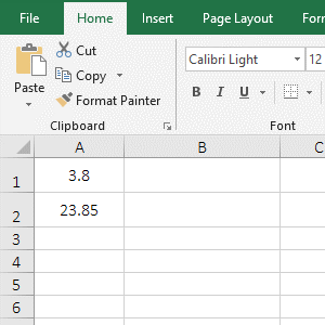
Figure 2
2. Formula description:
A. The format of the formula =TEXT(A1,"0.0?") and =TEXT(A2,"0.0?") are 0.0?, the question mark(?) in the format is used to fill spaces, that is, add a space before and after 3.8 in A1 to the same digit as 23.85 in A2 to align their decimal points.
(III) Do not display 0 on the left of the decimal point
1. Double-click the cell B1, copy the formula =TEXT(A1,"#.00") to B1, press Enter, return to .38; double-click A1, change 0.38 to 2.38, and the value in B1 becomes 2.38; the process steps are shown in Figure 3:
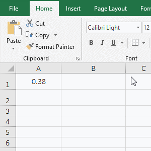
Figure 3
2. Formula description:
As you can see from the demo, when the number to the left of the decimal point is less than 1, the format #.00 returns the result of omitting the left side 0 of the decimal point; when the value to the left of the decimal point is greater than or equal to 1, the format returns the result of retaining the value to the left of the decimal point.
(IV) The decimal is displayed as the fraction
1. If you want to change 2.5 to a fraction. Double-click the cell B1, copy the formula =TEXT(A1,"# 0/0") to B1, press Enter, return 2 1/2; double-click B1 again, change the format "# 0/0" to "# ? /?", press Enter, also return 2 1/2; the operation steps, as shown in Figure 4:
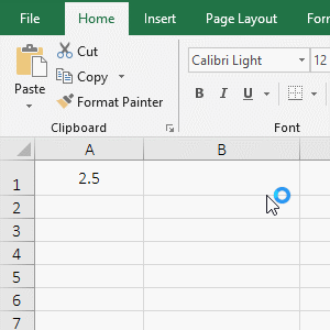
Figure 4
2. Formula description:
When changing decimals to fraction, you can use the format "# 0/0" or "# ?/?", that is, both the numerator and the denominator can be used with 0 or ?. In addition, if the numerator or denominator has multiple bits, you can use multiple 0(or ?), for example, to change 2.334 as a fraction, you can use the format "# ???/???".
(V) The numerical value is displayed as the format of thousands separator
1. If you want to add a comma to 2380000. Double-click the cell B1, copy the formula =TEXT(A1,"#,###") to B1, press Enter, return 2,380,000; double-click B1 and change the format "#,###" to "#,", press Enter, return to 2380; double-click B1, change "#," to "#.#,", press Enter, return to 2380; double-click B1 and change "#.#," to "#.#,, ", press Enter, return to 2.4; double-click B1 again, change "#.#,," to "0.0,," and return 2.4 again; the operation steps are as shown in Figure 5:

Figure 5
2. Formula description:
A. The format "#,###" indicates that a thousand separator(comic) is displayed every three digits from the single-digit of the value; the format "#," indicates that the digits of single-digit to hundred's place are omitted and rounded off. For example, 2380505 will become 2381.
B. The format "#.#," means to omit single-digit to hundred's place and round off to 1 decimal place; for example, 2380000 becomes 2380 in the demo.(# to the right of the decimal point will be omitted, as already mentioned above); format "# .#,," means to omit single-digit to hundred thousand and round off to 1 decimal place, such as 2380000 to 2.4 in the demo; format "0.0,," is the same as "#.#,,".
(VI) Examples of date formats
1. Double-click the cell B1, copy the formula =TEXT(A1,"yy/m/d") to B1, press Enter, return 19/10/8; double-click B2, copy the formula =TEXT(A1,"yyyy/mm/dd") to B2, press Enter, return to 2019/10/08; double-click B3, copy the formula =TEXT(A1,"yyyy/mmm/ddd") to B3, press Enter, return 2019/Oct/Tue; double-click B4, copy the formula =TEXT(A1,"yyyy/mmmm/dddd") to B4, press Enter, return to 2019/October/Tuesday; the operation steps are as shown in Figure 6:
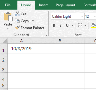
Figure 6
2. Formula description:
A. yy means that two digits are displayed in the year, m and d are both ones in the month and day in the format "yy-md". yyyy means that the year is four digits, and both mm and dd are two digits in "yyyy-mm-dd; If it is a single number, it is supplemented with 0.
B. mmm means that the month is displayed for the abbreviation of the word for the month, ddd means that the day is the abbreviation of the word for Monday to Sunday in the format "yyyy-mmm-ddd"; for example, returns 2019/Oct/Tue in the demo, Oct is a Abbreviation for October, Tue is an abbreviation for Tuesday.
C. mmmm means that the month is displayed for the word of the month, dddd means that the day is the word from Monday to Sunday in the format "yyyy-mmmm-dddd"; for example, returns 2019/October/Tuesday in the demo.
(VII) Examples of time formats
1. Double-click the cell B1, copy the formula =TEXT(A1,"h:m:s") to B1, press Enter, return to 15:6:9; double-click B2, copy =TEXT(A1,"hh:mm :ss") to B2, press Enter, return to 15:06:09; double-click A4, enter 23:66, double-click B4, copy the formula =TEXT(A4,"[h]:mm") to B4, press Enter, return 24:06; double-click B5, copy the formula =TEXT(A5,"[m]:ss") to B5, press Enter, return 119:06; double-click B6, copy the formula =TEXT(A6,"[s].00") to B6, press Enter, return 7146.50; operation steps, as shown in Figure 7:
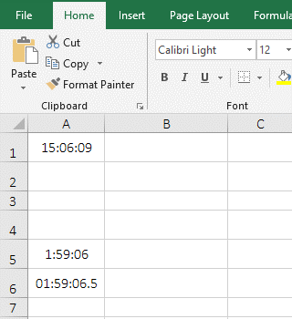
Figure 7
2. Formula description:
A. The format "h:m:s" means that only one bit is displayed in hours, minutes and seconds; "hh:mm:ss" means that both hours and minutes are displayed two digits, if there is only one bit, it is supplemented with 0.
B. The [h] in the format "[h]:mm" indicates that the time is displayed in hours. It can return the time when the number of hours exceeds 24, for example, 23:66(23 hours 66 minutes) returns 24:06(24 hours and 06 minutes) in the demo; [m] in "[m]:ss" means that the time is displayed in minutes, which can return the time of more than 60 minutes, for example, 1:59:06 returns 119:06(119 minutes and 06 minutes) in the demo; [s] in "[s].00" means that the time is displayed in seconds, which can return the time when the number of seconds exceeds 60, for example, 01:59:06.5 returns 7146.50(7146 seconds and 50 milliseconds).
3. If the time is to be expressed in AM or PM, the formula can be written as follows: =TEXT(A7,"hh:mm AM/PM").
(VIII) An example of adding a currency symbol before the value
1. If you want to add a dollar symbol($) to the "Price" column. Double-click the cell E2, copy the formula =TEXT(C2,"$0.0") to E2, press Enter, return to $1.3; select E2, move the mouse to the cell fill handle in the lower right corner of E2, and the mouse becomes the bold black plus. double-click the left button, and the remaining price is also added to $; the operation steps are as shown in Figure 8:
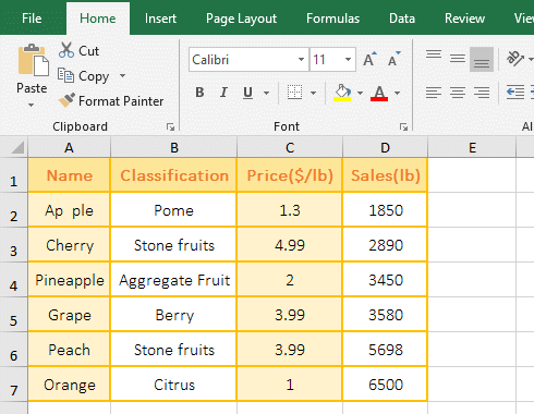
Figure 8
2. Formula description:
The input shortcut keys for currency symbols are: $(Shift + 4), cents (Alt + 0162), ££(Alt + 0163), and €€(Alt + 0128); you need to hold down Alt, The numbers are entered from the keypad, and the input method: hold down Alt, enter number on the NumLock, then release Alt.
(IX) Display a percent(%)
1. Double-click the cell B1, copy the formula =TEXT(A1,"0.00%") to B1, press Enter, return to 36.54%; select B1, move the mouse to the cell fill handle in the lower right corner of B1, and after the mouse changes to the bold black plus, double-click the left button, then the remaining value is also added %; the operation steps, as shown in Figure 9:
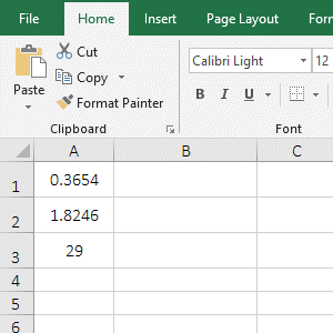
Figure 9
2. Formula description:
The formula = TEXT(A1,"0.00%") has the format "0.00%", which means that the value is rounded up to two decimal places and the percent is added; both the decimal and the integer are expanded by 100 times and added the percent and both are rounded up to two decimal places from the demo.
(X) Represented by scientific notation
1. Double-click the cell B1, copy the formula =TEXT(A1,"0.0E+0") to B1, press Enter, return to 5.8E+9; double-click B2, copy the same formula to B2, enter 0 after 0.0E+0, press Enter to return to 5.8E+09; double-click B3, copy the formula =TEXT(A3,"0.0E+0") to B3, press Enter, return to 5.7E+8; double-click B4, the formula in B3 is copied to B4, then the 0 before the decimal point is changed to #, press Enter, and return to 5.7E+8; the operation steps are as shown in Figure 10:
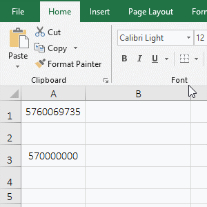
Figure 10
2. Formula description:
A. The difference of the formula =TEXT(A1,"0.0E+0") and =TEXT(A1,"0.0E+00") is that after the plus(+) in the format is less than 0 and more than 0, which is actually the definition, Whether the leading 0 is displayed when the exponent is less than two digits.
B. The formula =TEXT(A3,"0.0E+0") and =TEXT(A3,"#.0E+0") return the same result, and their difference is: the former is represented by 0 before the decimal point, the latter is represented by # before the decimal point, indicating that there can be both 0 and # before the decimal in the format.
C. It is known that when expressed in scientific notation, it is automatically rounded off from the results returned from A1 and A3.
III, The extended application examples of Excel Text function
(I) Use the placeholders # and * to convert numbers to text and round up
1. If you want to convert the sales volume to the text and round it up. Double-click the cell E2, copy the formula =TEXT(D2,"#*,") to E2, press Enter, return to 1851; convert the other values to text and round up with the method of double-clicking the cell fill the handle; the operation steps are as shown in Figure 11:
Figure 11
2. Formula =TEXT(D2,"#*,") explanation:
The # represents a number, * means any number of characters, "," is a thousand separator in the format "#*,", "#*," means that all numbers are converted to text and only rounded up integer.
(II) Format with conditions
1. If the sales volume is greater than 0, returns it; if the sales volume is equal to 0 or is empty, returns 0. Double-click the cell E2, copy the formula =TEXT(D2,"[>"&$D$4&"]0") to E2, press Enter, return to 638; returns the remaining results with double-clicking the cell fill handle; Then double-click F2, copy the same formula to F2, then enter ";z!ero" after the format, press Enter, return 638, double-click the cell fill handle to return the result of the remaining cells; the operation steps are as shown in Figure 12:
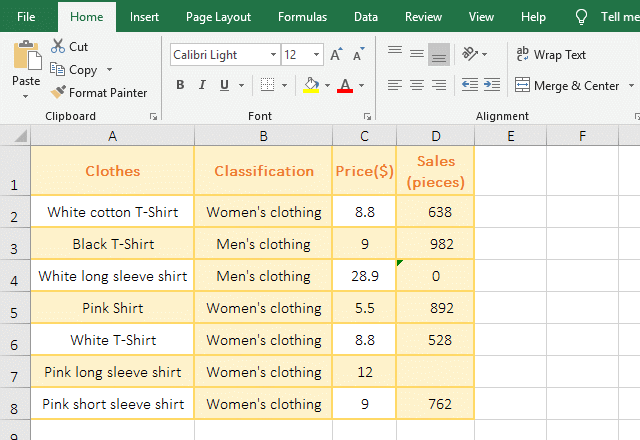
Figure 12
2. Formula =TEXT(D2,"[>"&$D$4&"]0") explanation:
A. $D$4 is 0, $ represents an absolute reference to the column and row to ensure that D4 does not become D5, D6, etc. when dragging down.
B. The format "[>"&D4&"]0" becomes "[>0]0", [>0] is the condition, 0 is the value that is displayed when the condition is met, and 0 in the format is a placeholder instead of refers to itself.
C. The formula becomes = TEXT(D2,"[>0]0"), meaning that if D2 is greater than 0, the placeholder 0(ie D2) is displayed, otherwise the 0 is displayed by default(if another value is defined, then this value is displayed); which can be confirmed by the formula =TEXT(D2,"[>"&$D$4&"]0;z!ero"), when the formula is in F2, D2 is greater than 0, it returns the value 638 in D2; when the formula is in F4, D4 is 0, which returns "zero. Because "e" is a placeholder, so add ! before it.
D. In addition, the ! is added in format "[>0]!0" after the last 0, the meaning is exactly the opposite of "[>0]0", meaning that if D2 is greater than 0, the placeholder 0 is not displayed, but 0 is displayed.
(III) Comparison of two positive and negative numbers, 0, empty cells and text format
1. If you want a positive number is rounded up to 1 decimal place, a negative number is returned empty, 0 and an empty cell are returned 0, the text is returned 0 or itself. Double-click the cell B2, copy the formula =TEXT(A2,"0.0;;0;!0") to B2, press Enter, return to 2.0; select B2 again, move the mouse to the cell fill handle in the lower right corner of B2, after the mouse becomes the bold black plus, double-click the left button to return the result of the remaining cells; double-click C2, copy the same formula to C2, delete ";!0" in the formula, press Enter, return 2.0 as well, and drag down to return other results; the operation steps are as shown in Figure 13:
Figure 13
2. Formula description:
A. There are four formats in the format "0.0;; 0;! 0", the first type "0.0;" means to round up to 1 decimal place; the second ";" means to return negative numbers as empty text; the three "0;" means that 0 and the empty cell are returned to 0; the fourth "!0" means to convert the text to 0, which is from the formula =TEXT(A7,"0.0;;0;!0") and =TEXT(A7,"0.0;;0") for the return value of A7; there is "!0", return 0; there is no "!0", return excel.
B. In addition, if there is no text in the value, you can omit "!0" in the formula =TEXT(A7,"0.0;;0;!0").
(IV) Condition range format
1. If the sales volume is greater than or equal to 5000 or less than 4000, returns the value, otherwise returns empty text. Double-click the cell E2, copy the formula =TEXT(D2,"[>=5000]0;[<4000]0;;") to E2, press Enter, return 1850; returns the result of remaining value with the method of double-clicking the cell fill handle; double-click F2, copy the formula =TEXT(D2,"[>=5000]!Hi!g!h; [<4000]Low;!M!e!diu!m") to F2, press Enter, return to "Low", and then double-click the cell fill handle of to return other results; the operation steps are as shown in Figure 14:
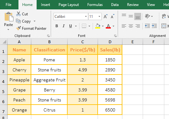
Figure 14
2. Formula description:
A. The format consists of four parts in the formula =TEXT(D2,"[>=5000]0;[<4000]0;;"), "[>=5000]0;" means that the value is greater than or equal to 5000, returns itself, 0 is the placeholder; "[<4000]0;" means that the value is less than 4000, returns also itself; ";" means that the value is from 4000 to 5000, returns empty text.
B. The formula =TEXT(D2,"[>=5000]!Hi!g!h; [<4000]Low;!M!e!diu!m") is the same as =TEXT(D2,"[>=5000]0;[<4000]0;;"), only However, the text is used instead of the value.
Tip: If you want to display special symbols(such as: placeholders 0, #, *, !, @, E, e, M, m, H, h, G, g, /), you need to add a exclamation point(!), otherwise it will return a value or value error #VALUE!, the demonstration shows in Figure 15:
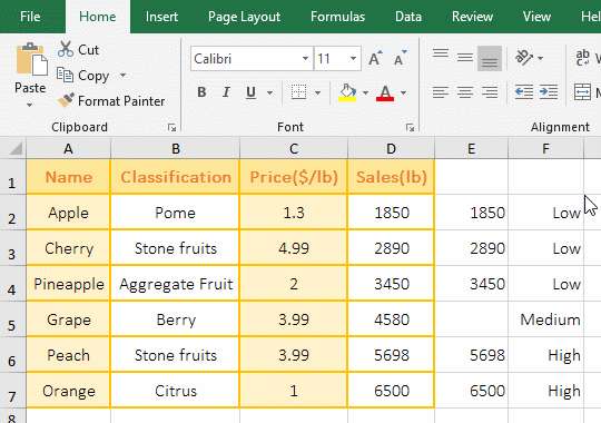
Figure 15
(V) The value is an array {0,1} or {-1,1}
(1) The format is two single values
1. Double-click the cell F2, copy the formula =TEXT({0,1},D2&";"&E2) to F2, press Enter, return to 20; double-click F2, change 0 to 1, press Enter, return to 21, select F2, move the mouse to the cell fill handle in the lower right corner of F2, after the mouse changes to +, hold down the left button and drag to F3, F3 returns 22; double-click F2, change the left 1 to 5, press Enter, return to 25; double-click F2, change 5 to 1, 1 to -1, press Enter, return to 21; double-click F2, change 1 to -1, -1 to 1, press Enter, return to 638; the operation steps are as shown in Figure 16:
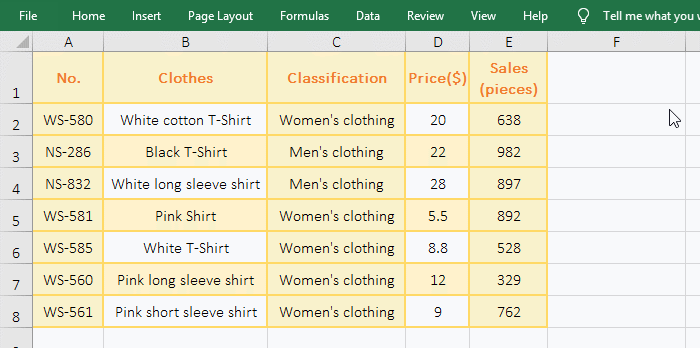
Figure 16
2. Formula description:
(A) =TEXT({0,1},D2&";"&E2)
A. {0,1} is a numeric argument in the formula, it is an array with only two elements; D2&";"&E2 is a format argument, which is consisted of D2, ";" and E2; 0 in the array {0,1} is a placeholder instead of itself.
B. Why does the formula only return D2(ie 20) without returning E2? First, 0 corresponds to D2, and 1 also corresponds to D2 in {0,1}, because the elements in the array are greater than 0 and correspond to D2, only the elements are less than 0 to correspond to E2, so E2 is not returned; 0 is a placeholder, so it returns 20; secondly, because you want to return an array, you need to put =TEXT({0,1},D2&";"&E2) in the referenced function, otherwise only return the first value, so the value corresponding to 1 is not returned, as shown in the following section "Format is an array".
(B) =TEXT({1,1},D2&";"&E2) and =TEXT({5,1},D2&";"&E2)
A. Both 1 correspond to D2 in the array {1,1} and only return D2, but why return 21 instead of returning 20? When D2 is a numeric type and the single-digit of D2 is 0, 1 in {1,1} will be added to D2, otherwise 1 in {1,1} will not be added to D2, so 21 is returned, which is confirmed from dragging F2 down to F3 from the demo, because D3(22) does not return 23.
B. In addition, when D2 is text, if 0 is on the right side of the number, then 0 will be replaced by 1, such as 130 to change 131; if 0 is on the left side of the number, 0 will be also replaced by 1, such as 013 to 113; if left and right of the number are 0, then only 0 on the right is replaced by 1, such as 0130 to 0131; the demo is shown in Figure 17:
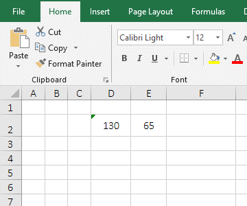
Figure 17
C. When the first element in the array {5,1} is 5, D2 will also add 5, and so on.
(C) =TEXT({1,-1},D2&";"&E2) and =TEXT({-1,1},D2&";"&E2)
A. 1 corresponds to D2, -1 corresponds to E2 in the array {1,-1}; and -1 also corresponds to E2, 1 corresponds to D2 in {-1,1}, because -1 is the first element of the array, thus returning E2(ie 638).
B. Tip: If E2 is 630, then 630 will also increase by 1 and become 631. It can be seen that when -1 is the first element of the array, D2 will swap the position with E2 and will add the absolute value of -1 to E2, if you want to know more, you can see "Format as an array" below; if E2 is text, it is the same as D2 is text.
(2) Format is an array
1. If you want to find the sales volume with the price of 198. Double-click the cell F2, copy the formula =IFERROR(VLOOKUP(198,--TEXT({0,1},D2:D8&";"&E2:E8),2),"") to F2, press Ctrl + Shift + Enter, return to 198; double-click F3, copy the formula =IFERROR(VLOOKUP(198,--TEXT({1,-1},D2:D8&";"&E2:E8),2),"") to F3, Press Ctrl + Shift + Enter, return to 991; double-click F4, copy the formula =IFERROR(VLOOKUP(198,--TEXT({-1,1},D2:D8&";"&E2:E8),1),"") to F4, press Ctrl + Shift + Enter, return empty text; the operation steps are as shown in Figure 18:
Figure 18
2. Formula description:
(A) =IFERROR(VLOOKUP(198,--TEXT({0,1},D2:D8&";"&E2:E8),2),"")
A. D2:D8 returns the values in D2 to D8 as an array, which returns {"80";"82";"88";"90";"89";"80";"198"}; E2:E8 is the same as D2:D8, it returns {"973";"899";"920";"1250";"995";"680";"990"}.
B. D2:D8&";"&E2:E8 becomes {"80";"82";"88";"90";"89";"80";"198"}&";"&{"973";"899";"920";"1250";"995";"680";"990"}, when the formula is executed, the first elements are taken from the two arrays for the first time and connect them together, that is, "80;973"; the second elements are taken from the two arrays, and they are also connected, that is, "82;899"; the others and so on, and return finally {"80;973";"82;899";"88;920";"90;1250";"89;995";"80;680";"198;990"}.
C. Then TEXT({0,1},D2:D8&";"&E2:E8) becomes TEXT({0,1},{"80;973";"82;899";"88;920";"90;1250";"89;995";"80;680";"198;990"}):
First execution: Take the first element "80;973" from the format array
First, take 0 from {0,1}, since the element in {0,1} is greater than 0, only return the element to the left of each element of the format array (such as returning only 80 of the first element "80;973" without returning 973); and because the first element 0 in {0,1} is a placeholder, it returns 80.
Second, take 1 from {0,1}, because 1 also corresponds to 80, and because the elements in {0,1} are greater than 0 and the single-digit of the element in the format array is 0, the value in {0,1} + the value in the format array is returned, so returning 80 + 1, returns 81.
Second execution: Take the second element from the format array "82;899"
First, take 0 from {0,1}, and return 82.
Second, take 1 from {0,1} and because the single-digit of 82 is not 0, do not add 1, so return 82.
Others and so on, and return finally {"80","81";"82","82";"88","88";"90","91";"89","89";80","81";"198","198"}.
D. Then --TEXT({0,1},D2:D8&";"&E2:E8),2) becomes --{"80","81";"82","82";"88","88";"90","91";"89","89";80","81";"198","198"}, then convert the elements in the array from text to numeric values, -- is the same as Value function, its function is that converts text to a value, returns finally {80,81;82,82;88,88;90,91;89,89;80,81;198,198}.
E. Then the formula becomes =IFERROR (VLOOKUP(198,{80,81;82,82;88,88;90,91;89,89;80,81;198,198}, 2), ""), further calculation, lookup 198 in the first column of the array (the column of comma "," to the left) with VLookUp function, find it on the last row, and then return the value 198 corresponding to 198 in the second column.
The function of IfError function is: If VLookUp returns the correct value, IfError returns the value, otherwise IfError returns null.
(B) =IFERROR(VLOOKUP(198,--TEXT({1,-1},D2:D8&";"&E2:E8),2),"")
The formula and the above formula are a meaning, except that the array {1,-1} is different. Only the array is analyzed below:
A. From the above analysis, D2:D8&";"&E2:E8 returns {"80;973";"82;899";"88;920";"90;1250";"89;995";"80;680";"198;990"}.
B. Then TEXT({1,-1}, D2:D8&";"&E2:E8) becomes TEXT({1,-1},{"80;973";"82;899";"88;920";"90;1250";"89;995";"80;680";"198;990"})
First execution: Take the first element "80;973" from the format array
First, 1 is taken from {1,-1}, since 1 corresponds to 80, it returns 80 + 1, which returns 81; secondly, -1 is taken from {1,-1}, since -1 corresponds to 973, it returns 973.
Second execution: Take the second element from the format array "82;899"
First, 1 is taken out from {1,-1}, since 1 corresponds to 82, so it returns 82; secondly, -1 is taken from {1,-1}, and since -1 corresponds to 899, it returns to 899.
Others and so on, and return finally {"81","973";"82","899";"88","921";"91","1251";"89","995";"81","681";"198","991"}.
(C) =IFERROR(VLOOKUP(198,--TEXT({-1,1},D2:D8&";"&E2:E8),1),"")(the difference between formats {1,-1} and {{ -1,1})
From the above analysis, TEXT({-1,1}, D2:D8&";"&E2:E8) becomes
TEXT({-1,1},{"80;973";"82;899";"88;920";"90;1250";"89;955";"80;680";"198;990"}).
First execution: Take the first element "80;973 from the format array
First, take -1 from {-1,1}, since -1 corresponds to 973, it returns 973; secondly, 1 is taken out from {-1,1}, since 1 corresponds to 80, it returns 80 + 1, which returns 81.
Second execution: Take the second element "82;899" from the format array
First, take -1 from {-1,1}, since -1 corresponds to 899, it returns 899; secondly, 1 is taken out from {-1,1}, and since 1 corresponds to 82, it returns to 82.
Others and so on, and return finally {"973","81";"899","82";"921","88";"1251","91";"995","89";"681","81";"991","198"}.
From the above analysis, the difference between the format {1,-1} and {-1,1} is: when -1 is on the right, the right value of each element of the format array is returned to the right, equivalent to if{0,1}; when -1 is on the left, the value of the right side of each element of the format array is returned to the left, equivalent to if{1,0}; for if{1,0}, please refer to the article "Vlookup with if statement(use if/if{0,1} combination two or three conditions)".
-
Related Reading
- How to use Excel Trim function(6 examples, with lead
- How to use Excel Right function and RightB(8 example
- VLookUp in excel introduces step by step(10 examples
- Excel If function examples, include if statement nes
- How to find duplicate values in excel using vlookup(
- Excel SumIf function with ?/*, Average and array mul
- Excel substitute function usage(8 examples, with mul
- How to use Excel clean function(5 examples, with non
- Vlookup with if statement(use if/if{0,1} combination
- Excel averageif function usage(7 examples, include R
- Excel Choose function usage(it and Vlookup, Match co