 Office > Excel > Excel 2019 > Content
Excel substitute function usage(8 examples, with multiple characters,nest,vba,quantity in formula)
The Substitute function is used to replace one character or a string of characters with another character or a string of characters in Excel. If the characters to be replaced have multiple identical characters, not only can all characters be replaced, but also the first few character that is specified can be replaced. Replace function is also used for replacement, which differs from the Substitute function at the end of the article.
The Substitute function can be used in combination with IsText, Sum, Value, Evaluate, etc., and can also be nested. For example, Evaluate + Substitute + Substitute + IsText combination implements quantity calculation, Sum + Value + Substitute combination can add the values with unit, Substitute nests to replace multiple characters.
I, The syntax of Excel Substitute function
1. Expression: SUBSTITUTE(Text, Old_Text, New_Text, [Instance_Num])
2. Description:
A. Substitute function is used to replace the specified old characters with one or a new string of characters. If the characters to be replaced have the same, you can use the argument Instance_Num to specify which one to replace; if Instance_Num is 1, replace the first one, the other and so on. If Instance_Num is omitted, all the same characters are replaced.
B. Substitute function does not support the wildcard question marks(?) and asterisks(*), for example, the * in Old_Text or New_Text does not represent any one or more characters, only * itself.
C. Substitute function is case sensitive. For example, there are "ab" and "Ab" in the Text, if the only writes "ab" in Old_Text, "Ab" is not replaced.
II, The examples of Excel Substitute function
(I) Replace all the same characters
1. If you want to replace all the "lb" in the D column. Double-click the cell D2, copy the formula =SUBSTITUTE(D2,"lb","") to D2, press Enter, return to the number 1850; select D2, move the mouse to the cell fill handle in the lower right corner of D2, after the mouse becomes the bold black plus, double-click the left button, then the "lb" in the remaining digits of column D is also replaced; the operation steps are as shown in Figure 1:
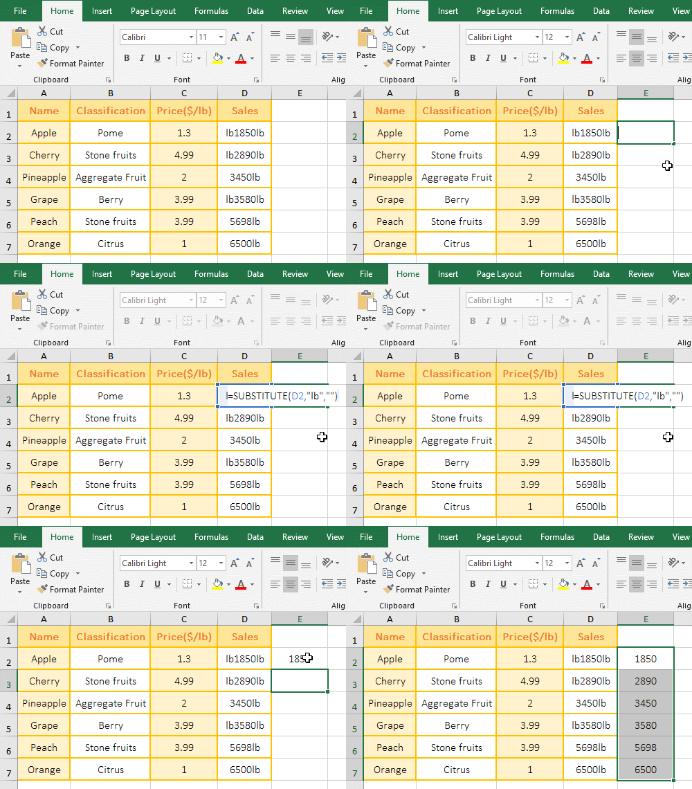
Figure 1
2. Formula description:
D2 is the Text, "lb" is the Old_Text, "" is the New_Text, the last argument Instance_Num is omited, the default Replace all "lb" in the formula =SUBSTITUTE(D2,"lb",""); the formula means: replace all the "lb" in D2 with the empty text "".
(II) Replace only the specified same character
1. If only the second "lb" in the D column is replaced. Double-click the cell D2, copy the formula =SUBSTITUTE(D2,"lb","",2) to D2, press Enter, return to "lb1850" which only the second "lb" is replaced; the operation steps are as shown in Figure 2:
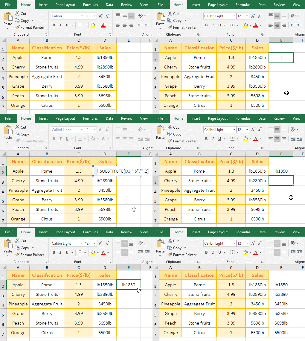
Figure 2
2. Formula description:
The formula =SUBSTITUTE(D2,"lb","",2) compared with the formula of the above example, there is only the fourth argument 2, meaning: Replace the second "lb" in D2 with the empty text "", from the returned result "lb1850" shows that only the second "lb" is replaced, the first one is not replaced; D3 is the same as D5 and D2, and the other cells are only one "lb", and are not replaced.
(III) ? and * are not wildcards
1. Double-click the cell B1, copy the formula =SUBSTITUTE(A1,"d*","") to B1, press Enter, return to the number 78969759389231
which the "d*" are replaced; double-click B2, copy the formula =SUBSTITUTE(A2,"?","0") to B2, press Enter, return to the 25802765093802378
which "?" is replaced with 0; the operation steps, as shown in Figure 3:
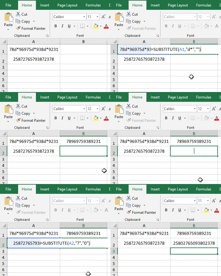
Figure 3
2. Formula description:
A. The * in the "d*" only represents itself in the formula =SUBSTITUTE(A1,"d*",""), if it represents any character, then all characters after "d" are replaced, indicating the function Substitute does not support the wildcards *.
B. The replaced character in the formula =SUBSTITUTE(A2,"?","0") is ?, which also represents itself. If it represents any character, the first digit in A2 should be replaced.
(IV) The example of case-insensitive replacement
1. If you want to replace the "word" in "word 2019, Word 2016, word 2013" with "excel". Double-click the cell A2 cell, copy the formula =SUBSTITUTE(A1,"word","excel") to A2, press Enter, return to "excel 2019, Word 2016, excel 2013"; the process steps, as shown in Figure 4:
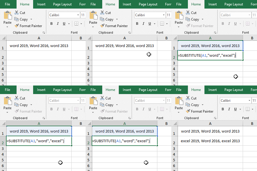
Figure 4
2. As you can see from the replacement result, "Word" starting with uppercase "W" is not replaced, and both lowercase words are replaced, indicating that the Substitute function is case sensitive.
(V) Replace only a single numerical instance
1. If you want to replace the individual 2 in "20,2,23,16,36,2,28,52", you cannot replace 2 such as 23. Double-click the cell B1, copy the formula =SUBSTITUTE(A1,",2,",",") to B1, press Enter, return to the result "20,23,16,36,28,52" which 2 are replaced; the steps are as shown in Figure 5:
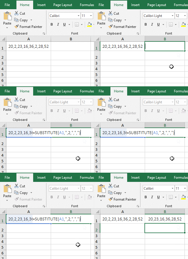
Figure 5
2. Formula description:
The replaced text is ",2," in the formula =SUBSTITUTE(A1,",2,",","), and there are commas before and after the 2, which is mainly used to distinguish 2 such as 23, if only write "2", then all 2 of A1 are replaced.
III, The application example of Excel Substitute function
(I) Excel substitute multiple characters instances: The nested of the Substitute function to replace multiple different characters at a time
1. If you want to replace the left and right double quotes and spaces in column A. Double-click the cell D2, copy the formula =SUBSTITUTE(SUBSTITUTE(A2," ",""),"""","") to D2, press Enter, the double quotes and space in A2 are replaced; select D2, replace the double quotes of the remaining cells by using double-click the cell fill handle; the operation steps are as shown in Figure 6:
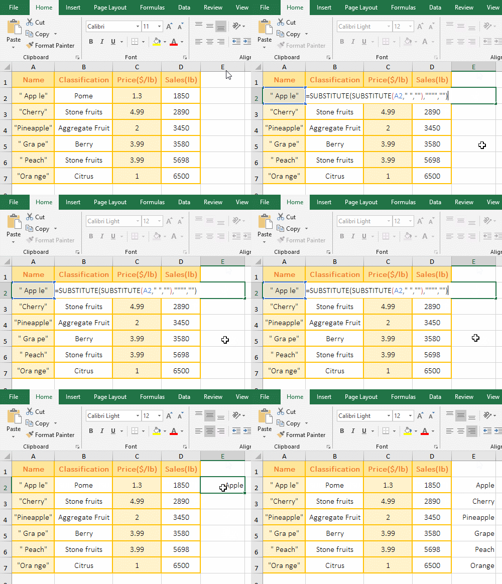
Figure 6
2. Formula =SUBSTITUTE(SUBSTITUTE(A2," ",""),"""","") description:
A. The inner layer SUBSTITUTE(A2," ","") is used to replace the spaces, it returns the result "Apple".
B. The formula becomes =SUBSTITUTE("""Apple""","""",""), and finally replaces the double quotation mark(") with a space, and the double quotation marks on both the left and right sides of A2 are replaced.
(II) Sum + Value + Substitute combination to add the values with units
1. There is a fruit sales table, with units of "lb" after sales, and now they need to be summed. Double-click the cell D8, copy the formula =SUM(VALUE(SUBSTITUTE(D2:D7,"lb",""))) to D8, press Ctrl + Shift + Enter to return the summation result 23968; double-click D8, change VALUE to --, press Enter, and return the same result; the process steps, as shown in Figure 7:
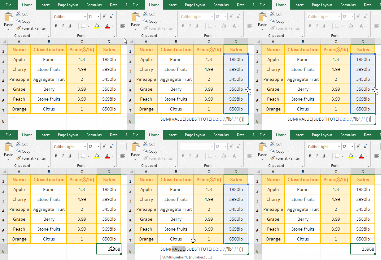
Figure 7
2. The formula =SUM(VALUE(SUBSTITUTE(D2:D7,"lb",""))) description:
A. The formula is an array formula, so press Ctrl + Shift + Enter; D2:D7 returns all the values in D2 to D7 as an array.
B. Then SUBSTITUTE(D2:D7,"lb","") becomes SUBSTITUTE({"1850lb";"2890lb";"3450lb";"3580lb";"5698lb";"6500lb"},"lb",""), then, take the first element "1850lb" from the array, then replace the "lb" with the empty text "", and so on, and finally return {"1850";"2890";"3450";"3580";"5698";"6500"}.
C. Then VALUE(SUBSTITUTE(D2:D7,"lb","")) becomes VALUE({"1850";"2890";"3450";"3580";"5698";"6500"}), further calculations, use Value to convert each element in the array to a value; -- as with Value.
D. The formula becomes =SUM(1850;2890;3450;3580;5698;6500), and finally adds the elements in the array.
(III) Substitute + Substitute + IsText combination calculates quantity
(1) Calculated by definition name
1. If you want to calculate the volume of the wall. Select cell A2 where the calculation formula is located, select the "Formula" tab, click the "Definition Name", open the "New Name" window, enter "qua" after "Name", select "Sheet1" for "Scope", copy the formula =IFERROR(EVALUATE(SUBSTITUTE(SUBSTITUTE(Sheet1!$A$2,"[","*ISTEXT(""["),"]","]"")")),"") to the input box to the right of "Refers to", click "OK", the name definition is completed; select B2, enter =qua, press Enter, return to the calculation result 7.68; the operation process steps, as shown in Figure 8:
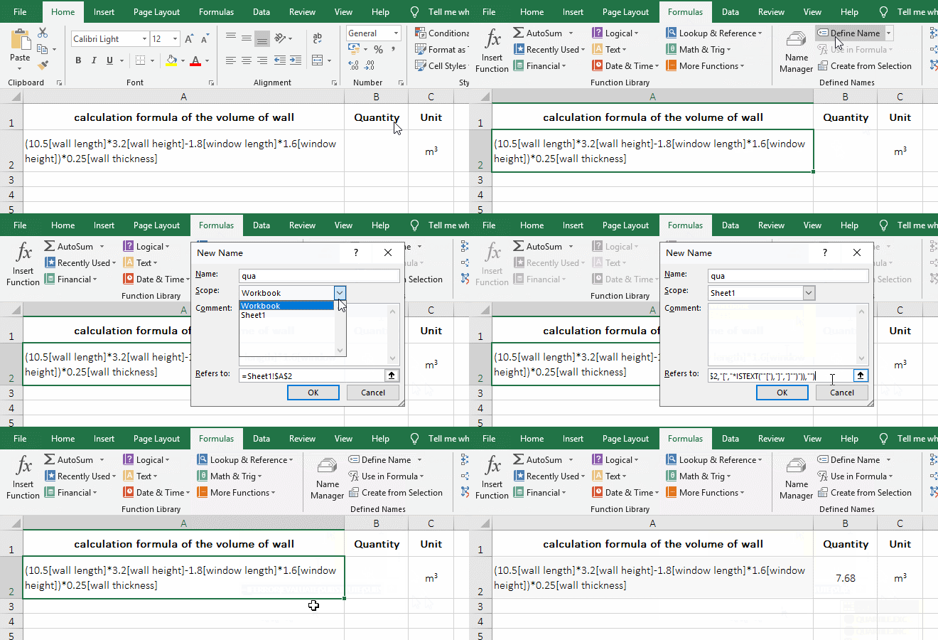
Figure 8
2. Formula =IFERROR(EVALUATE(SUBSTITUTE(SUBSTITUTE(Sheet1!$A$2,"[","*ISTEXT(""["),"]","]"")")),"") explanation:
A. Sheet1!$A$2 is an absolute reference to the A2 cell in Sheet1. When the name is defined, the cell needs an absolute reference, otherwise it will find no cell.
B. The most inner layer of the formula SUBSTITUTE (Sheet1!$A$2,"[","*ISTEXT(""[") is used to replace all left brackets [ in A2 with *ISTEXT(""[;, the purpose is to use the IsText function to determine whether the comment following the number in A2 is text, and if so, return True(ie 1), otherwise return False(ie 0); for example, IsText("[wall height]") returns True.
Tip: When replacing double quotes, use two double quotes, for example, replaces [ with *ISTEXT(""[, because you need to add a double quote before [, so adds two double quotes in *ISTEXT(""[.
C. Then SUBSTITUTE(SUBSTITUTE(Sheet1!$A$2,"[","*ISTEXT(""["),"]","]"")") becomes SUBSTITUTE("(10.5*ISTEXT("[wall length]*3.2*ISTEXT("[wall height]-1.8*ISTEXT("[window length]*1.6*ISTEXT("[window])*0.25*ISTEXT("[wall thickness]","]", "]"")"), then, replace ] with "]").
D. The formula becomes =IFERROR(EVALUATE("(10.5*ISTEXT("[wall length]")*3.2*ISTEXT("[wall height]")-1.8*ISTEXT("[window length]")*1.6 *ISTEXT("[window]"))*0.25*ISTEXT("[wall thickness]")"),""), further calculation, use Evaluate to execute a replacement "calculation formula of the volume of wall", due to each IsText Both return 1, so the formula becomes =IFERROR(EVALUATE("(10.5*1*3.2*1-1.8*1*1.6*1)*0.25*1"),"").
E. Further calculation, the formula becomes =IFERROR(7.68,""). Since 7.68 is not an error value, the IfError function returns 7.68; the IfError function is used for error judgment. If Evaluate returns an error, IfError will return "", otherwise it returns the return value of Evaluate.
(2) Calculated with macro(VBA, Excel vba substitute string)
1. Also take the calculation of the wall volume as an example. In the Excel window, press Alt + F11 to open the VBA editing window, click "Insert", select "Module" in the pop-up menu, create a new module, and copy the following code:
Public Sub Test()
[B3] = EVALUATE(Application.Substitute(Application.Substitute([B2],"[","*ISTEXT(""["), "]","]"")"))
End Sub
To the module, click "Run", select "Run Sub/User Form" in the pop-up menu, the calculation is completed and output the result 7.68 to the cell B3, press Alt + F11 again to switch to the Excel window to see; the operation process steps are as shown in Figure 9:
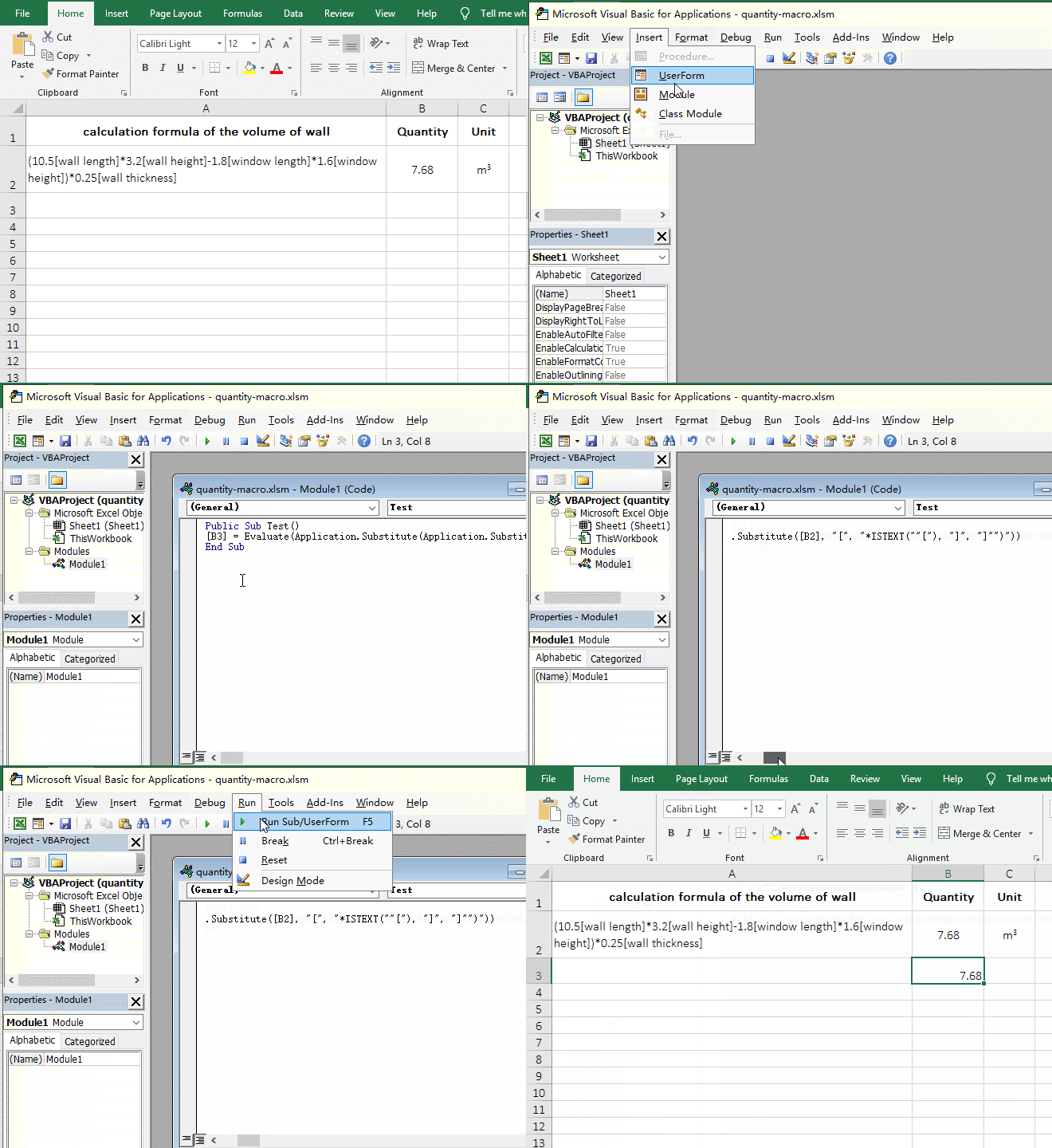
Figure 9
2. VBA code description:
A. [B2] means to reference the cell B2. To reference a cell in VBA, enclose it in square brackets [].
B. When using a function in VBA, you need to add "Application." in front of it, otherwise you will be prompted to find no the function, such as Application.Substitute.
C. [B3] is used to output the execution result of Evaluate, so after executing the code, there is 7.68 in B3.
Tip: For the above two quantity calculation methods, when saving, "Save as type" needs to select "Excel Macro-Enable Workbook", otherwise it will not be executed correctly next time.
IV, The difference between the Replace function and the Substitute function
The Replace function replaces a certain number of characters with the specified characters, the Substitute function replaces another(or a string of characters) with one(or a string) character; the Replace function is mainly used to replace a long string of characters at a time, and the Substitute function is mainly used to replace one word with another. If you want to replace one word with another or replace a long string of characters with empty text(""), use two functions to achieve the following:
1. If you want to replace "Excel" with "Word" in A1. Double-click the cell B1, copy the formula =REPLACE(A1,1,4,"Excel") to B1, press Enter, return to "Excel table technique"; double-click B2, and copy the formula =SUBSTITUTE(A1,"Word","Excel") to B2, press Enter, and return also to "Excel table technique".
2. If you want to replace a long string of messy characters in A4 with empty text. Double-click B4, copy the formula =REPLACE(A4,FIND("8",A4),FIND("4 fun",A4)-FIND("8",A4)+2,"") to B4, press Enter, return to "Excel function tutorial"; then double-click B5, copy the formula =SUBSTITUTE(A4," 8ut43it-r*753iot9oyt5trey8345fdh4","") to B5, press Enter, also return "Excel function tutorial"; operation process steps, As shown in Figure 10:
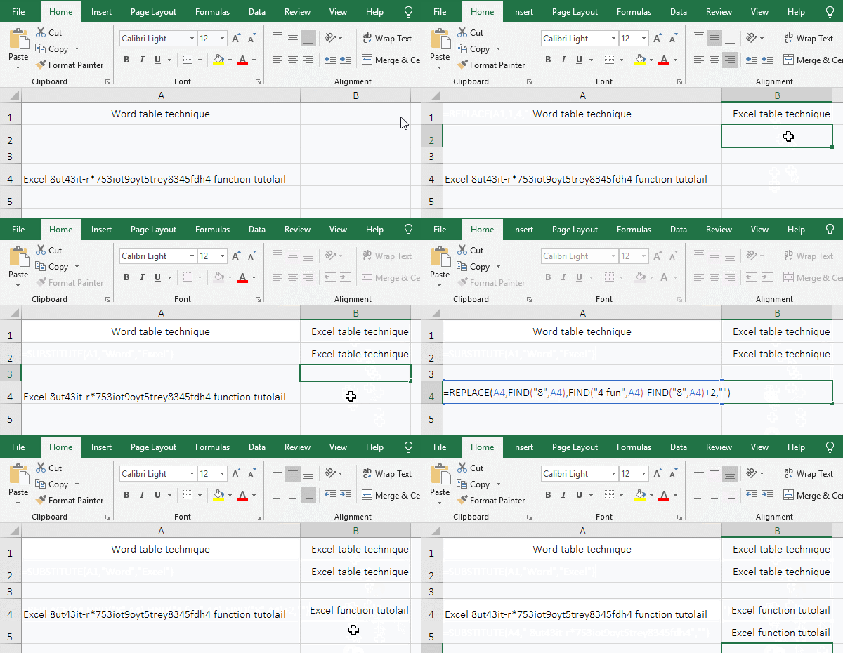
Figure 10
3. Formula description:
A. The Formula =REPLACE(A1,1,4,"Excel") means to replace 4 characters with "Excel" from the first character in A1, that is, to replace "Word" in A1, "Word" is exactly 4 characters. The formula =SUBSTITUTE(A1,"Word","Excel") replaces "Word" in A1 directly with "Excel"; as you can see from the two formulas, the latter formula is simpler.
B. The formula =REPLACE(A4,FIND("8",A4),FIND("4 fun",A4)-FIND("8",A4)+2,"") means, replaces 34 characters with empty text ("") from the 7th in A4, which happens to be the messy character and the last space in A4.
FIND("8",A4) returns the position of the first character(ie 8) of the string to be replaced in A4, resulting in 7.
FIND("4 fun",A4)-FIND("8",A4)+2 is used to calculate the number of characters to be replaced, which is to use the last position of the characters to be replaced subtract the position of first character of characters to be replaced and add 2, add 2 is also to replace the space after the string that is replaced.
FIND("4 fun",A4) is used to return the position of the last letter of the characters to be replaced in A4, the result is 39, the reason is to find "4 fun" because there is more than one 4 in A4 to avoid mistakes.
C. The formula =SUBSTITUTE(A4," 8ut43it-r*753iot9oyt5trey8345fdh4","") replaces directly " 8ut43it-r * 753iot9oyt5trey8345fdh4" with "", the formula is simpler than using the Replace function, but it is very inconvenient to replace the particularly long characters when you write the formula.
-
Related Reading
- Excel Len and LenN function usage(7 examples, with I
- Excel Search function and SearchB usage(13 examples,
- Excel CountA and CountBlank function usage examples(
- How to use Replace function in excel(9 examples, wit
- 8 examples of Excel Match function, include it and S
- How to use offset function in excel, include it and
- Excel SumProduct function(multiple criteria, with if
- Excel left function usage(8 examples, with Sum+Value
- How to use Average function in excel(combine with if
- Excel Mid function and Midb usage(6 examples, includ
- How to use Excel Right function and RightB(8 example
- How to use Excel address function(7 examples, with I