Excel Choose function usage(it and Vlookup, Match combination to performance evaluation in formula)

The excel Choose function is used to select the value specified by the index number from the list of values. Its index number ranges from 1 to 254, and at least one, at most 254. The index of the Choose function can be numbers, arrays, functions and formulas; values can be cells, definition names and formulas, in addition to numbers.

The Choose function can be used in combination with functions such as VLookUp, Match, and Sum, in addition to returning a value; for example, VlookUp + Choose for reverse lookup, Choose + Match for performance or score evaluation.

I, Excel Choose function syntax

1. Expression: CHOOSE (Index_Num, Value1, [Value2], ...)

2. Description:

A. Index_Num can be a numeric value, an array, a reference to a cell, and a formula, but the value, array and value in cell, and returned value of the formula must be between 1 and 254. If Index_Num is less than 1 or greater than the number of reference lists, the Choose function will return the value error #VALUE!.

B. If Index_Num is 1, the Choose function returns Value1; Index_Num is 2, and the Choose function returns Value2; others and so on.

C. If Index_Num is a decimal, only the integer part is truncated, and the fractional part is completely discarded and not rounded.

D. Choose function must have at least one Value, at most 254: Value can be a number, a reference to a cell, a defined name, a formula, a function, or a text.

II, The examples of Excel Choose function

(I) Index_Num is a numeric value and returns #VALUE!

1. Double-click cell A8, copy the formula =CHOOSE(4,A2,A3,A4,A5) to A8, press Enter to return to the "Pineapple"; double-click A8 again, change 4 to 0, press Enter, return Value error #VALUE!; Double-click A8, change 0 to 5, press Enter, and also return the #VALUE!; operation process steps, as shown in Figure 1:

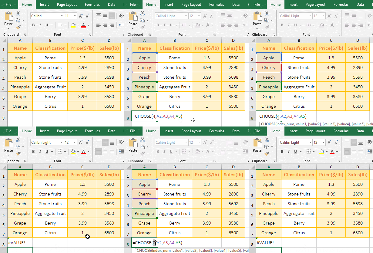
Figure 1

2. Formula description:

4 is the index number in the formula =CHOOSE(4,A2,A3,A4,A5), and A2, A3, A4, and A5 are values. The formula means: the fourth value is selected from A2, A3, A4, and A5, select A5(Pineapple); change 4 to 0 and 5 are beyond the range of Index_Num(The range of Index_Num is greater than 0 and less than or equal to the number of reference lists, there are only 4 values in the formula, so The number of lists is 4), so the return value is incorrect #VALUE!.

(II) Index_Num is a decimal

1. Double-click the cell E8, copy the formula =CHOOSE(3.6,C2,C3,C4,C5) to C8, press Enter, return to 3.99; the operation steps, as shown in Figure 2:

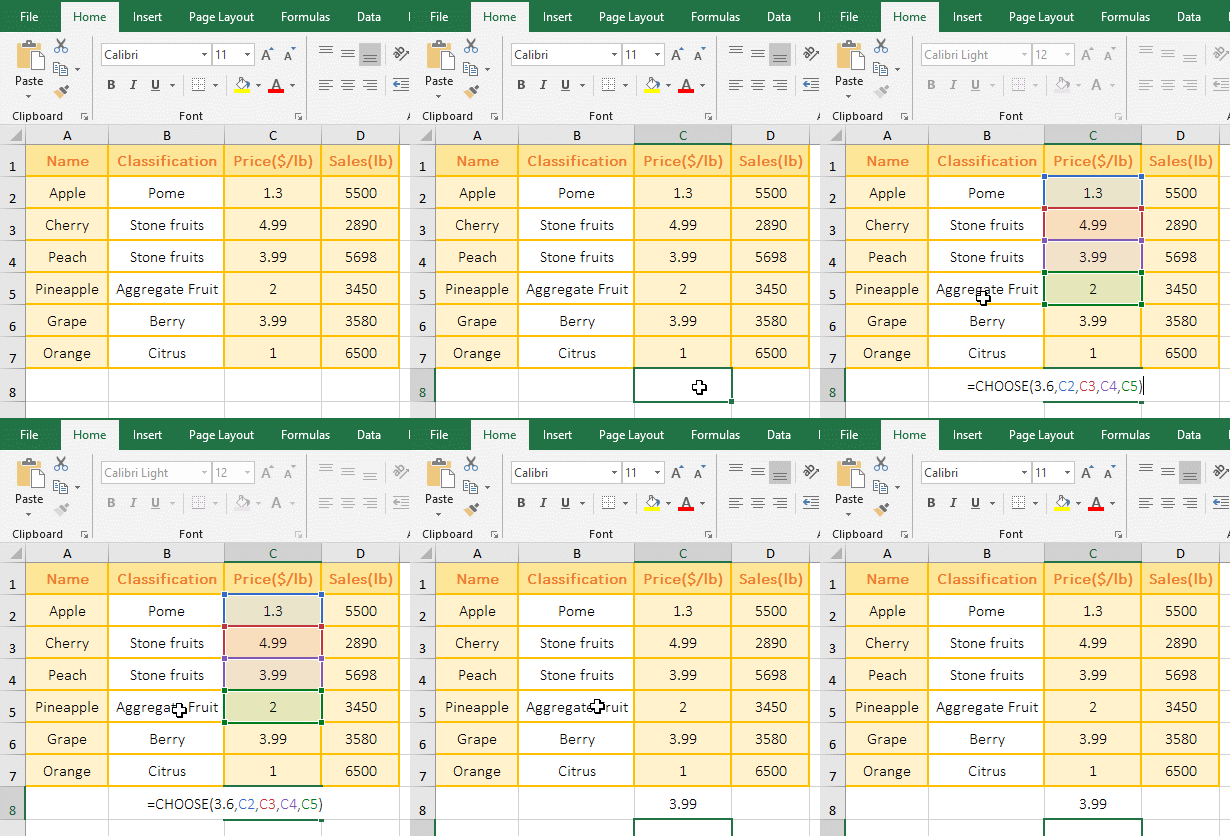
Figure 2

2. 3.99 that was returned by formula =CHOOSE(3.6,C2,C3,C4,C5) is exactly the value in C4, indicating that 3.6 is rounded to 3.

(III) A reference to cells returns only the value in cell that is the same row as the formula

1. Double-click the cell E2, copy the formula =CHOOSE(1,C2:C7)) to E2, press Enter, return to 1.3; select E2, move the mouse to the cell fill handle in the lower right corner of E2, and after the mouse becomes bold black plus, hold down the left button, drag down until you drag to E4, F3 and F4 return 4.99 and 3.99 respectively; double-click the cell D8, copy the formula =CHOOSE(1,C2:C7)) to D8, press Enter, return Value error #VALUE!; the operation steps are as shown in Figure 3:

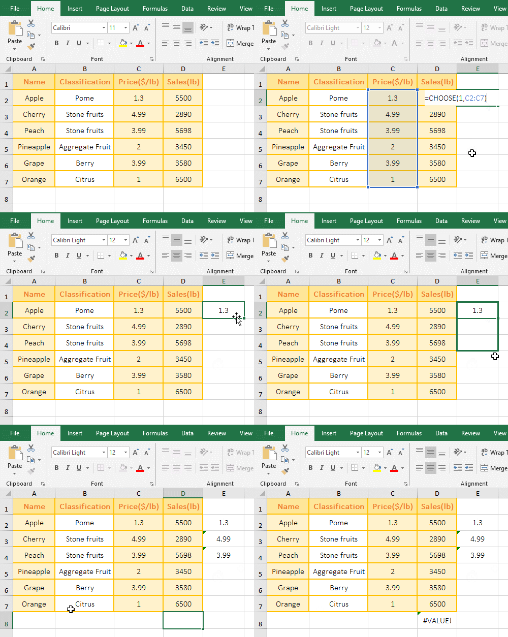
Figure 3

2. When the formula is in the cells F2 to F4, it returns the corresponding value on the same row as them. For example, when the formula is E2, it returns the value in C2 on the same row as E2; when the formula is copied to D8, the returned value is error #VALUE!, when the reference to a range, the Choose function only returns the value in cell that is the same row as the formula.

Hint: If you want to return all the values of the referenced range, you need to put the Choose function into another function, for example, put it in the Sum function, such as =SUM(CHOOSE(1,C2:C7)), the result is the sum of C2 to C7.

III, The Excel Choose function extended use examples

(I) How to use choose function with vlookup in excel(reverse lookup; Choose's argument Index_Num is an array)

The detailed analysis of the VLookUp + Choose function combination has been introduced in the "VLookUp in excel introduces step by step(10 examples), include Reverse lookup,one-to-many lookup". Please click on the title of the article in the double quotes.

(II) Choose + Match function to achieve performance evaluation

1. If the sales performance of the salesperson is to be assessed, it is assumed that the sales amount below 40,000 is poor, the 40,000 to 50,000 is qualified, the 50,000 to 60,000 is good, the 60,000 to 70,000 is excellent, and the above 70,000 is more excellent.

Double-click the cell D2 and copy the formula =CHOOSE(MATCH(C2,{0,40000,50000,60000,70000,100000}), "Poor", "Qualified", "Good", "Excellent", "More excellent") to D2, press Enter, return to "Poor"; select D2, move the mouse to the cell fill handle in the lower right corner of D2, after the mouse becomes the bold black plus, click the left button to return the performance evaluation of remaining salespersons; Operation process steps, as shown in Figure 4:

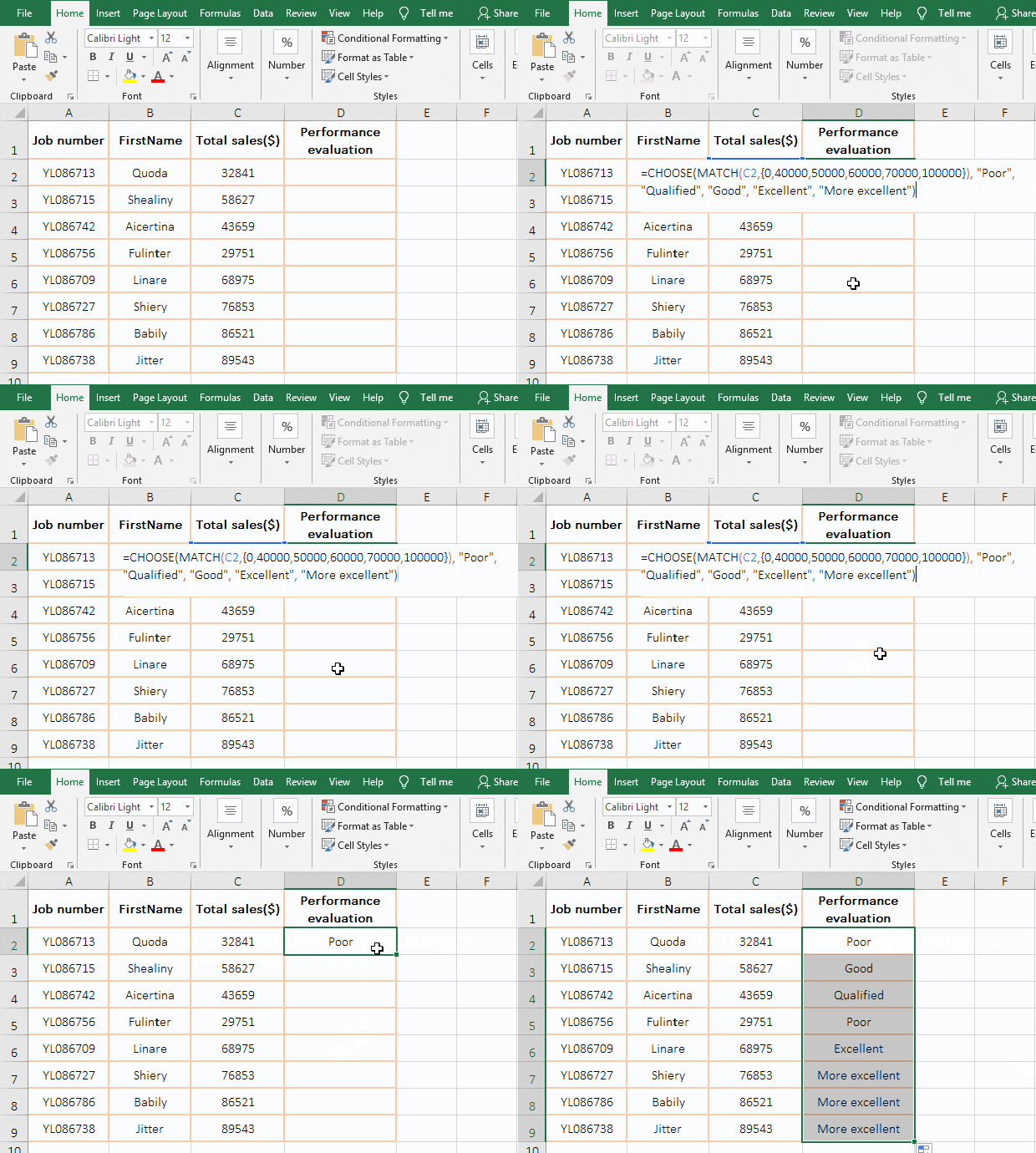
Figure 4

2. Formula =CHOOSE(MATCH(C2,{0,40000,50000,60000,70000,100000}), "Poor", "Qualified", "Good", "Excellent", "More excellent") desciption

A. MATCH(C2,{0,40000,50000,60000,70000,100000}) is used to return the position of C2(32841) in the array, the Match function omits the last argument, the default is 1, because there is no 32841 in the array, so return a value less than or equal to the lookup value, which returns 0, the position of 0 in the array is 1, so the Match function returns 1.

B. The formula becomes =CHOOSE(1, "Poor", "Qualified", "Good", "Excellent", "More excellent"), and then uses the Choose function to return the value of index number 1, which is "Poor" .

Tip: In addition to the Choose + Match function combination can achieve performance evaluation, LookUp function can also be, please see the "Approximate lookup"  in the article "Excel lookup function usage(Multiple conditional and approximate/fuzzy lookup)".

(III) Using the Definition Name as the value of the Choose function

1. Select B2:B8, select the "Formula" tab, click "Define Name", open the "New Name" window, "Name" keep the default " Blouse", click "OK"; select D2:D9, the same way to define the name "Trouser" for them; double-click the cell F2, enter the formula =CHOOSE(1,Blouse,Trouser), press Enter, return to 239, which happens to be the first value in B2:B9; double-click F2, change 1 to 2, press Enter, return to the first value of D2:D9; double-click F2 again, change the formula to =SUM(CHOOSE(2,Blouse,Trouser)), press Enter, return the sum of D2:D9; the operation process steps, as shown in Figure 5:

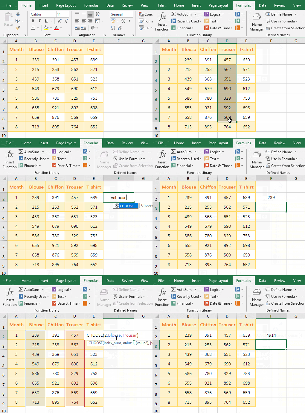
Figure 5

2. Description:

A. The argument value of the Choose function can be the name of the definition. In the formula, the Definition Name is not added with a double quotes, and the Chinese name is not added. For example, the "Blouse and Trouser" in the formula are not added.

B. When the Definition Name is a reference to a range, the default only returns the value that is the same row as the formula. The return value from the first argument of the Choose formula is 1 and 2 can explain this; if you want to return the all values contained by the Definition Name, you need to put Choose in another function. For example, put Choose in the Sum function and return the sum of D2:D9.

Hint: If you have more values and cannot be listed in the Choose function, you can also consider defining the value as a name.