How to use Excel clean function(5 examples, with non-printing characters that cann't delete)

The Clean function is used to remove all unprintable characters in the text in Excel. If these characters are before and after the text, you can delete them all; if they are between the characters or words, they will not delete all, but leave one. The Clean function works like the Trim function, except that the Trim function is used to remove the spaces.

The Clean function can only delete non-printing characters with ASCII code 0 to 31. Some non-printing Unicode characters cannot be deleted. This situation needs to be replaced with Substitute function; if it still cannot be deleted, you need to combine Left, Mid, Right, Code and other functions. In addition, Clean's text argument can be an array, this function can delete all the non-printing characters in one column at a time. If the summation value has non-printing characters, you need to remove them and then sum them with Clean.

I, The syntax of the Excel Clean function

1. Expression: ClEAN(Text)

2. Description:

A. Clean function is used to delete all non-printing characters in the text. These non-printing characters refer to characters encoded as 0 - 31 in the ASCII code table. Some of them are spaces, some of them are not. For details, please refer to the article "ASCII Table".

B. In addition to the non-printing characters in the ASCII code table, the Unicode character set also has non-printing characters, Their values are 127, 129, 141, 143, 144, and 157, the Clean function cannot delete them, To delete, you need to use Substitute function.

C. Argument Text is the text to delete non-printing characters; Clean function can delete all non-printing characters before and after the text, or delete non-printing characters between the text, but it will not delete all non-printing characters between the characters, it will leave one, which is the same as the Trim function used to remove spaces.

II, The examples of Excel Clean function

(I) Delete all non-printing character before and after the text

1. If you want to delete all non-printing characters before and after the text "    Excel Function Tutorial". Double-click the cell A1, copy the formula =CHAR(9)&"Excel Function Tutorial"&CHAR(11) to A1, select B1, enter the formula =CLEAN(A1), press Enter, return to "Excel Function Tutorial"; select A1:B1, press Ctrl + C to copy, switch to an empty Notepad window, press Ctrl + V to paste, all non-printing characters before and after the text in A1 are deleted; select "    Excel Function Tutorial", copy it to A2, enter the formula =CLEAN (A2) in B2, press Enter, and return to the "Excel function tutorial"; the operation process steps, as shown in Figure 1:

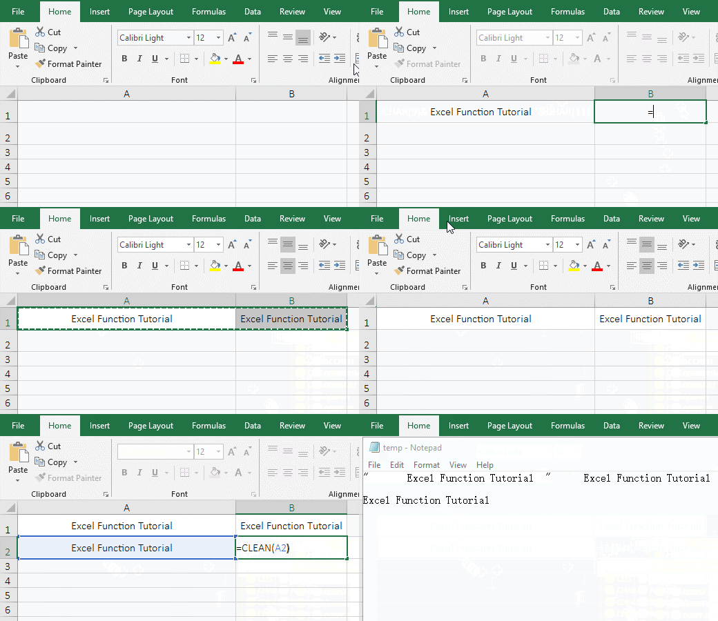
Figure 1

2. Description:

A. CHAR(9) returns "horizontal tab", 9 is the ASCII code of the horizontal tab; CHAR(11) returns "vertical tab", 11 is the ASCII code of the vertical tab.

B. the Clean function can delete both the non-printing characters returned by the Char function and the non-printing characters copied from the text to the cells from the above demonstration.

(II) Deleting non-printing character between words

1. If you want to delete the non-printing spaces in the text "Excel          Function Tutorial". Select the text to delete the space in the Notepad window, press Ctrl + C to copy, switch to the Excel window, double-click A1, press Ctrl + V to paste the text to A1, select B1, enter the formula =CLEAN(A1), press Enter, return to the "Excel function tutorial", there is still a space between the text, copy it back to the Notepad window and compare the original text; the process steps, as shown in Figure 2:

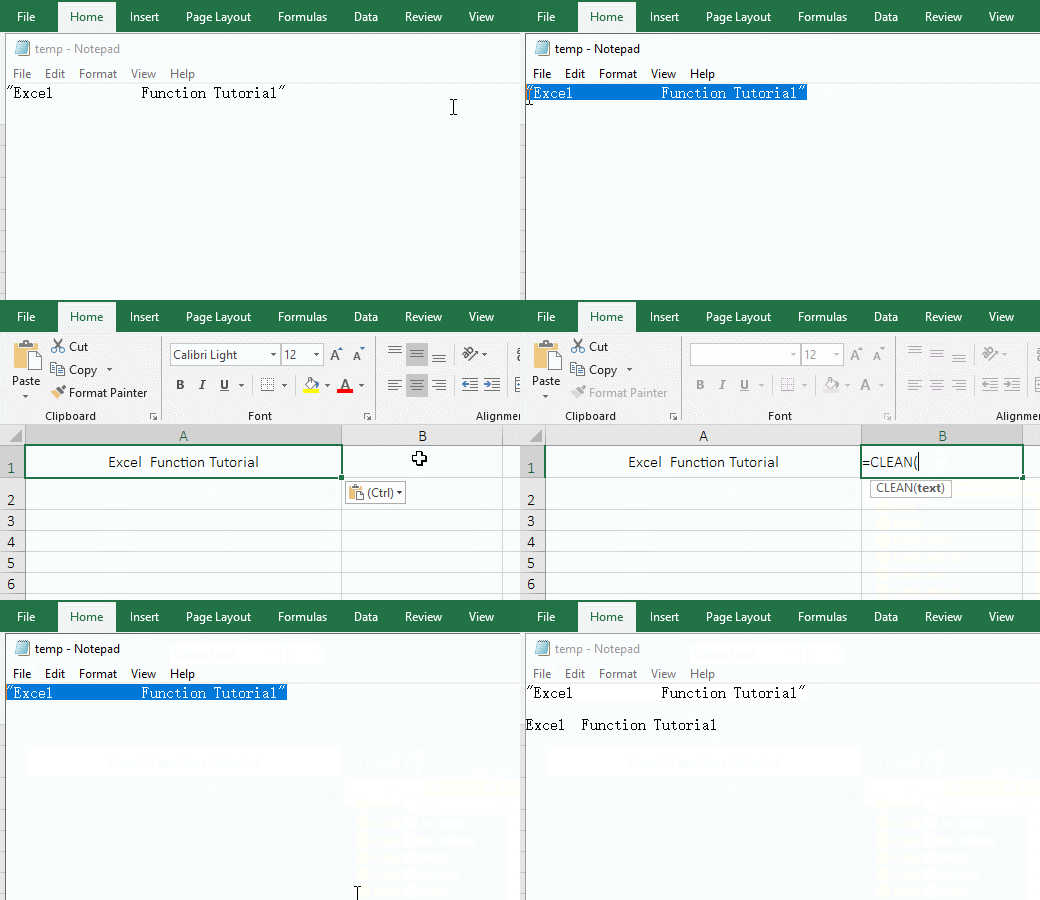
Figure 2

2. Formula description:

A. The formula =CLEAN (A1) can not delete the non-printing spaces in the "Excel          Function Tutorial", leaving one, if you want to delete the space, please use the following method.

III, The Excel Clean function can not delete the non-printing characters removal method

(I) Delete all spaces between characters

1. If you want to delete the spaces of "func  ti  on" in "Excel func  ti  on tutorial". Double-click the cell A1, select a space, press Ctrl + C to copy; select B1, enter the formula =SUBSTITUTE(A1,", press Ctrl + V to paste a space as the replaced character, then type "," "), press Enter, return the text "Excel function tutorial"; the operation steps are as shown in Figure 3:

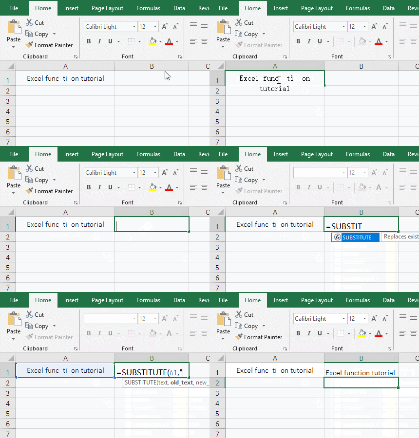
Figure 3

2. Formula =SUBSTITUTE(A1," ","") explanation:

The Substitute function is a replacement function that replaces one character or a string of characters with another character or another string of characters; A1 is the text to replace some characters, " " is replaced character, "" replaces the character in the formula =SUBSTITUTE(A1," ",""), the formula means: replace all " " with "" in A1.

(II) delete Unicode non-printing characters

Some Unicode non-printing characters can not be deleted by the Clean function, you also need to replace it with the Substitute function, as follows:

1. If you want to delete the character whose ASCII is 127 in the Unicode character set; double-click the cell A1, select the non-printing character behind the text, press Ctrl + C to copy, select B1, enter the formula =SUBSTITUTE(A1,", press Ctrl + V to paste the copied character, continue typing "," "), press Enter, all non-printing characters are deleted; double-click B2, copy the formula =SUBSTITUTE(A1,CHAR(127),"") to B2 , press Enter, all non-printing characters in A1 are also deleted; double-click A3, the non-printing characters indicated by CHAR(127), copy the formula =SUBSTITUTE(A3, CHAR(127),"") to B3, press Enter, all non-printing characters in A3 are also removed; the operation steps are as shown in Figure 4:

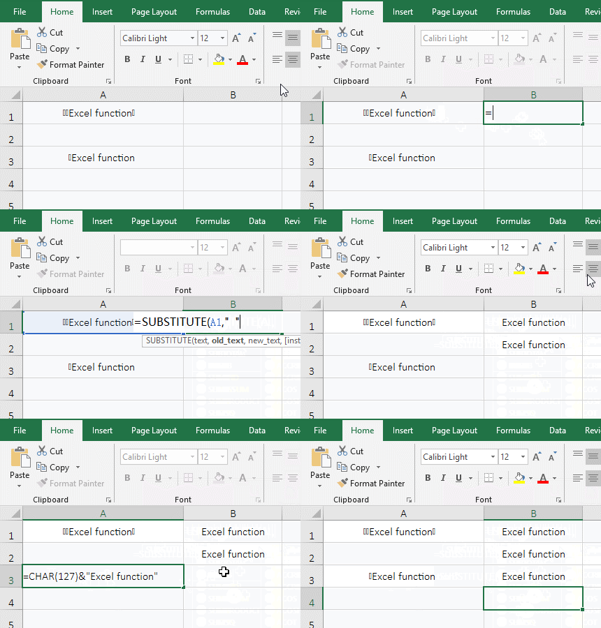
Figure 4

2. Formula description:

A. The formula =SUBSTITUTE (A1," ","") and =SUBSTITUTE(A1,CHAR(127),"") replace the non-printing characters whose ASCII code is 127 with the empty text ""; the difference between the two formulas is that the former copies the non-printing characters in A1 into the formula, the latter returns directly non-printing characters with CHAR(127).

B. The non-printing characters in A3 are returned with CHAR(127), you can also replace them with CHAR(127) as the replaced characters in the substitution formula =SUBSTITUTE(A3,CHAR(127),"").

Tip: If you can't delete non-printing characters by using the above method, you can use the Left, Mid or Right function to intercept a non-printing character as the replaced character, and then you can delete it. For details, please refer to the article "How to use Excel Trim function(6 examples, with leading,trailing,stubborn spaces and Left)".

IV, The extended application example of Excel Clean function

(I) Sum + Clean function combination adds the numbers with non-printing characters

1. If you want to sum the columns whose values are text and have non-printing characters in front. Double-click the cell D9, enter the formula =SUM(D2:D8), press Enter, return 0; double-click D9 again, change the formula to =SUM(VALUE(CLEAN(D2:D8))), press Ctrl + Shift + Enter, return the summation result 5,028; the operation process steps, as shown in Figure 5:

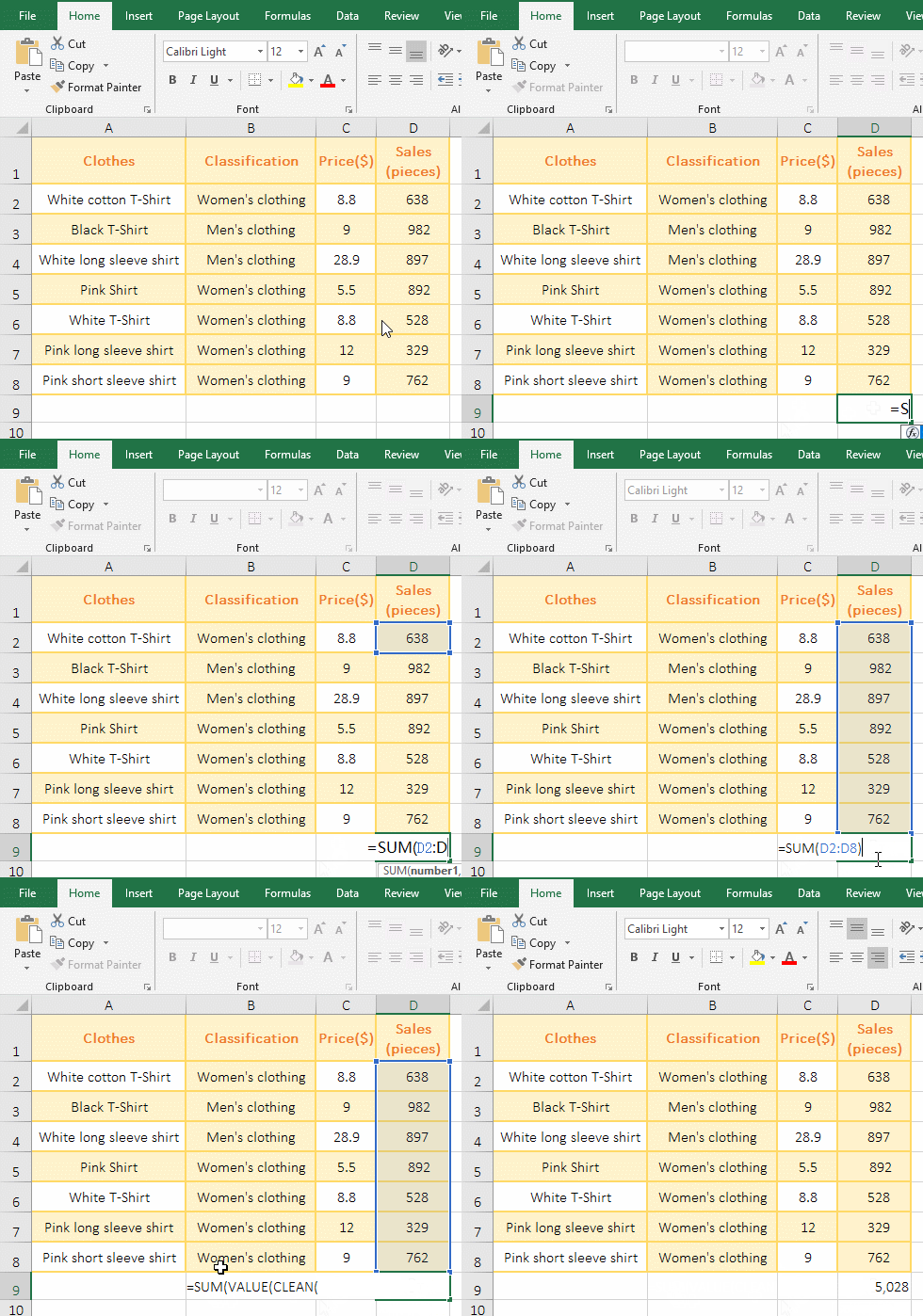
Figure 5

2. The formula =SUM(VALUE(CLEAN(D2:D8))) description:

A. The formula =SUM(D2:D8) returns 0 because the values in D2:D8 are preceded by non-printing characters. When calculating, the Sum function cannot convert them to numeric.

B. The formula =SUM(VALUE(CLEAN(D2:D8))) is an array formula, and the array formula needs to press Ctrl + Shift + Enter to return the calculation result.

C. D2:D8 returns all the values in D2 to D8 as an array. Then, the Clean function deletes the non-printing characters in front of each value, and finally returns the array {"638";"982";"897";"892";"528";"329";"762"}.

D. The formula becomes =SUM(VALUE({"638";"982";"897";"892";"528";"329";"762"})), further calculation, the all elements in array are converted  numeric values from text.

E. The formula becomes =SUM({638;982;897;892;528;329;762}), and finally the array is summed with the Sum function.

Hint: If you can't sum after one sum in D9, you need to set D9's cell format to "Number", press Ctrl + 1, open the "Format Cell" window, then select the "Number" tab, and finally select the "Number" on the left.