 Office > Excel > Excel 2019 > Content
How to split cells in excel, with unmerge cells and one column or a cell to two or mutiple columns
There are two ways to split a cell in Excel, one with the options provided by Excel and the other with shortcut. Excel split cells can only split the merged cells. You cannot split a single cell that has not been merged into two or more.
In addition to splitting cells, you often encounter splitting a cell into two or more cells or splitting a column into two or three columns or more in the process of editing an Excel table. Whether it is splitting the content of cell or splitting the column, you can use the Text to Columns and the formula; if the data has obvious separators or even distribution, you can use the Text to Columns; if the data is mixed with alphanumeric characters, you cannot use the Text to Columns, you can use the formula.
I, How to unmerge cells in excel
(1) Method 1: Selection method
Select the cells to be unmerge, such as A1 and B1, select the "Home" tab, click the black small inverted triangle to the right of "Merge & Center", and select "Unmerge cells" in the pop-up menu, then A1 and B1 are unmerged again; the process steps, as shown in Figure 1:
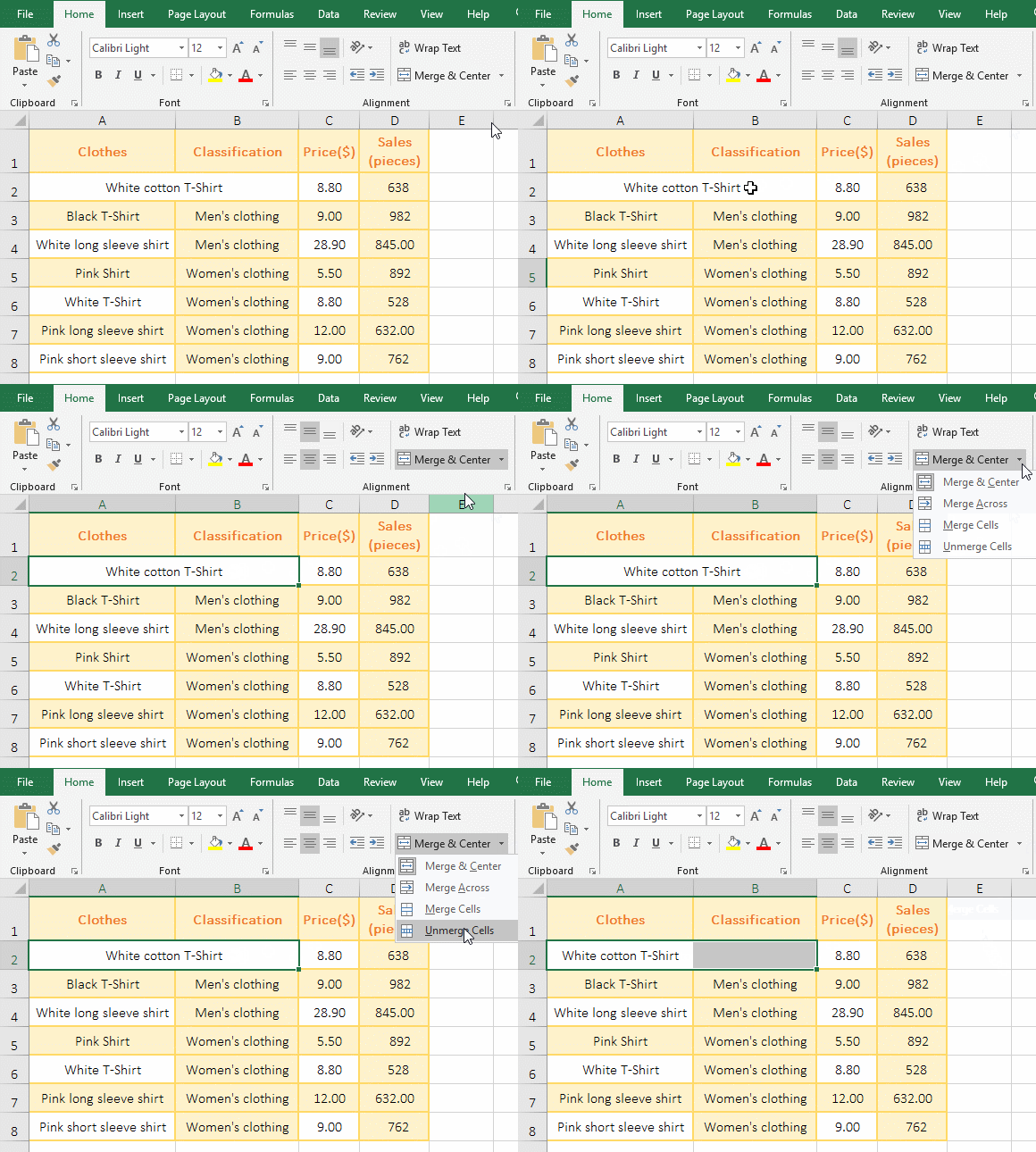
Figure 1
Hint: Excel split cells are not split into a few words like Word can be split, it will only be split according to the number of merged cells, for example, when merging cells is to merge two cells into one cell, then split it is automatically split into two; the three cells are combined into one cell, which is automatically split into three when splitting, and so on.
(2) Method 2: Shortcut method
Excel Unmerge Cells shortcut key is Alt + H + M + U, the operation method is: Select cells B3:C3, hold down Alt key, press H once, press M once, press U, then B3:C3 are Unmerged three cells again, the process steps, as shown in Figure 2:
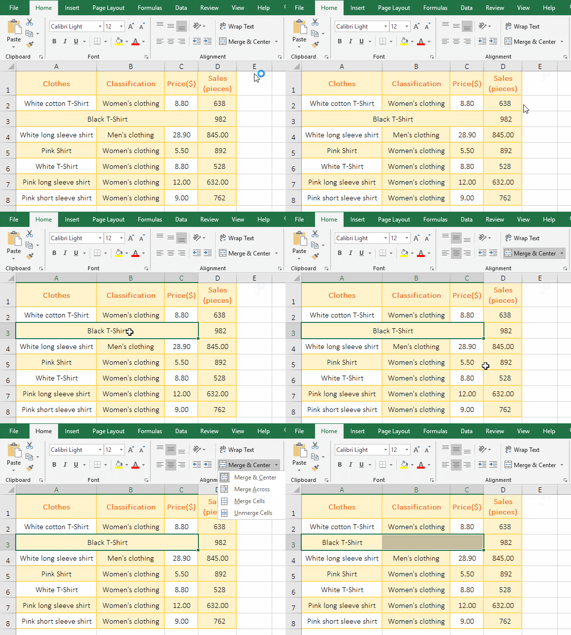
Figure 2
Hint: Since the cells to be Unmerged lacks a border, it looks like the three cells are still one, but the text has been moved to the cell A3; if you want to add a border to the cells to be unmerged, you can press Ctrl + 1 to open a dialog, select the "Border" tab, click the icon on the outerline, and click "OK".
II, How to split cells in excel(Split content)
(I) How to split a column into two in excel or how to split one cell into two in excel
1. If you want to split the "No." column of the clothing table into two columns. Right-click B at the top of the second column and select Insert from the pop-up menu. Insert a column between the first column and the second column; click A to select column A, select the "Data" tab, and click "Text to Column", open the "Convert Text to Columns Wizard" dialog, select "Delimited", click "Next", check "Other", enter - on the right side of "Other", click "Next", click "Finish", then the first column is split into two columns from the short cross(-); the operation steps are as shown in Figure 3:
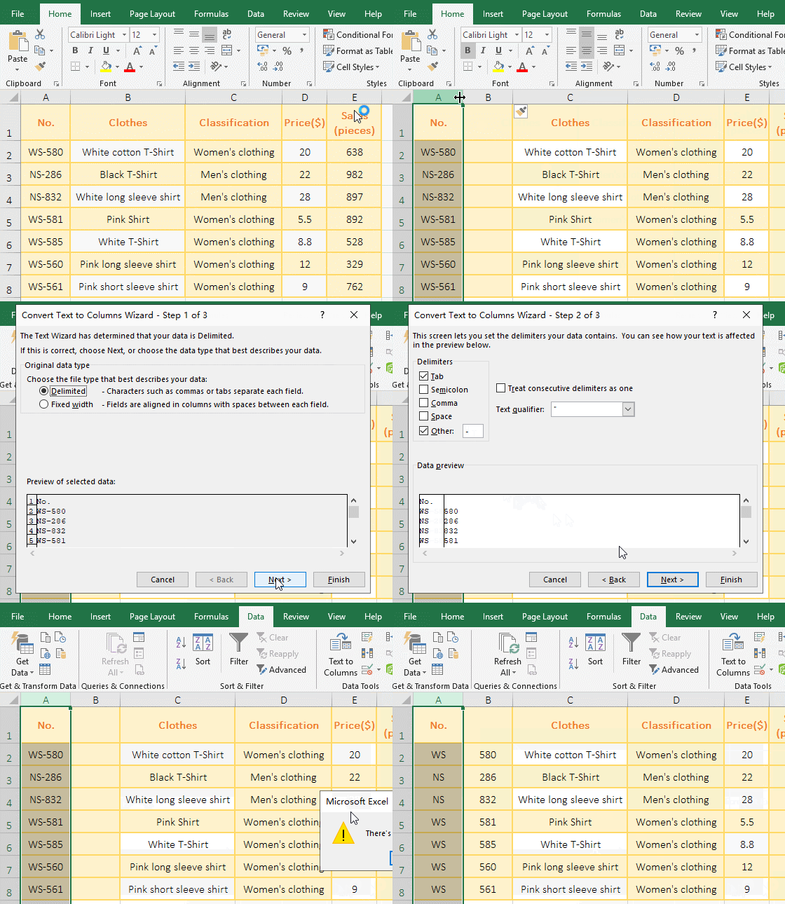
Figure 3
2. As can be seen from the split result, the split symbol(-) is not available after splitting, and the same is true if a character is used as a split character. In addition, there are four kinds of split characters in the "Convert Text to Columns Wizard", which are "Tab, semicolon, comma and space". If the content to be split is mostly one of the symbols, you can select it for splitting symbol.
(II) Splitting with "fixed width", which can be split into two or multiple columns(Excel split cell in half vertically)
1. Right-click the letter D in the column D, select "Insert" in the pop-up menu, insert a column to the right of the column D; select the column C, select the "Data" tab, click "Text to Column" to open the "Convert Text to Columns Wizard" dialog, select "Fixed Width", click "Next", move the mouse to the corresponding ruler where you want to split, click once, then an arrow pointing to the ruler appears, drag a little to the right so that the arrow is just at the point to be split, click "Next", the texts are split two pars and the left part is filled with the black background, you can confirm whether it is split as required; if it meets the requirements, Click "Finish"; If it does not meet the requirements, you can click "Back" to continue the adjustment; the split has been completed here, click "Finish", then one column is split into two columns; the operation steps are as shown in Figure 4:
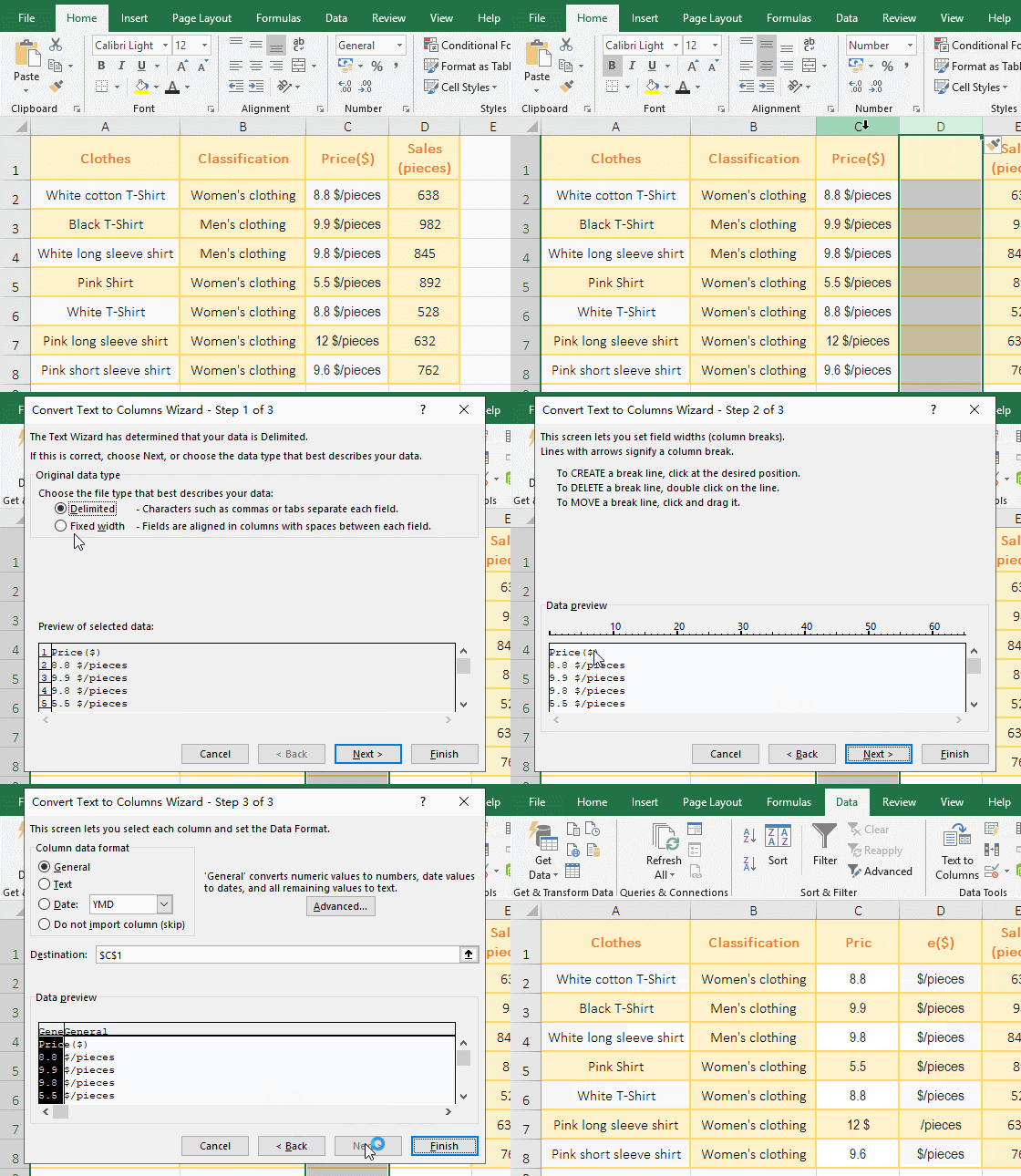
Figure 4
2. If you want to split into three columns, click one more time at the "ruler" of the "Convert Text to Columns Wizard" dialog, and then an arrow will appear again, and so on. The split of the Fixed Width applies to columns which data distribution is uniform and aligned.
(III) Excel split cell by delimiter formula(Suitable for columns with uneven data distribution)
1. Split the column with obvious delimiters(Excel split one cell into two)
(1) If you want to split the price column into a numeric column and a unit column. Select the cell E2, copy the formula =LEFT(C2,FIND("$",C2)-1) to E2, press Enter, return 8.8, then the number of price in C2 will be split to E2, and move the mouse the cell fill handle in the lower right corner of E2, hold down the left button and drag down, the number of other cells in the price column is also split into the corresponding cell of the column E; copy the formula =MID(C2,FIND("$",C2),8) to F2, press Enter, the unit of price in C2 is split to F2, and the unit of other cells in price column are split into column F by the method of dragging down; operation process steps, as shown in Figure 5:
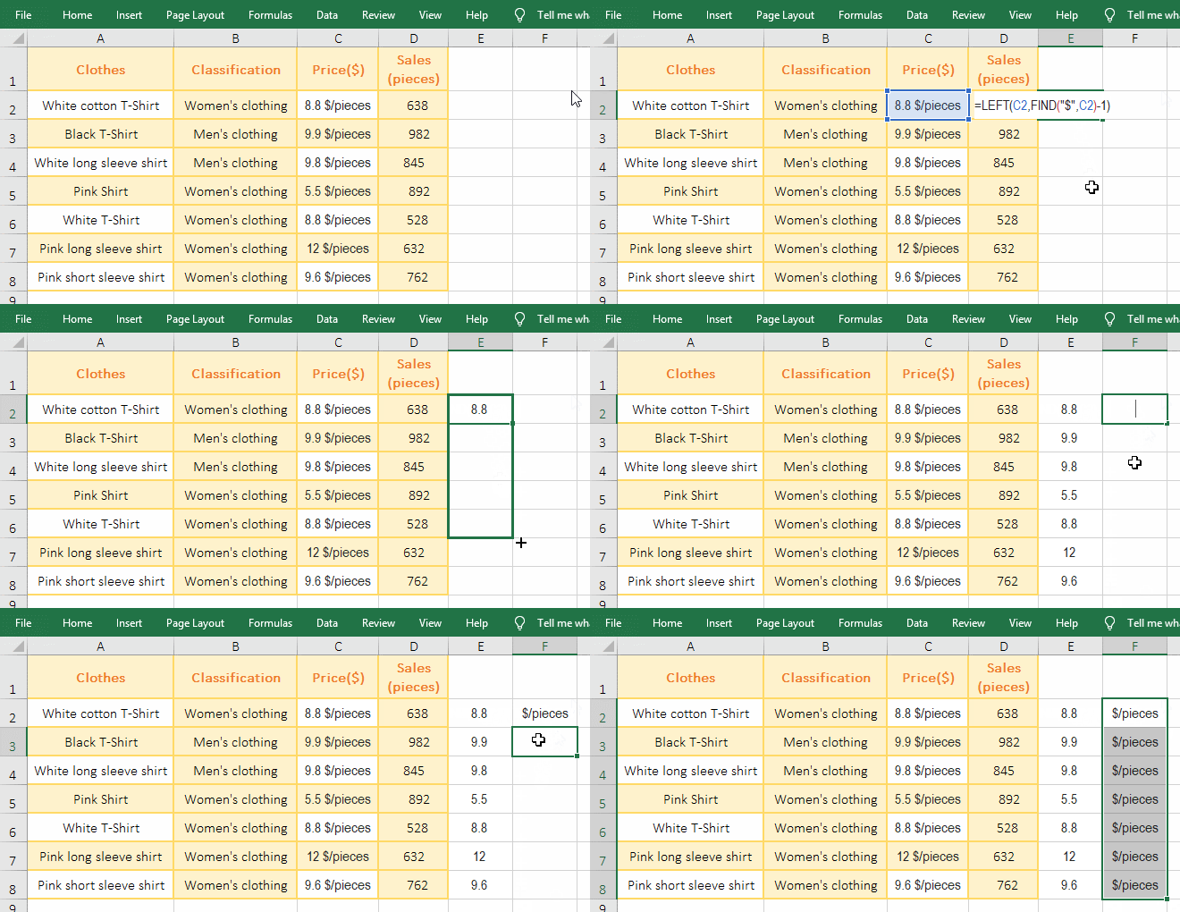
Figure 5
(2) Formula description:
A. The expression of the Left function is: =LEFT(Text,[Num_Chars]), Text is the source text, Num_Chars is the number of characters to be intercepted, it can be omitted;
The expression of the Find function is: =FIND(Find_Text,Within_Text,[Start_Num]), Find_Text is the text to be found, the Within_Text is source text, and Start_Num is the search start position, which can be omitted.
The expression of the Mid function is: =MID(Text,Start_Num,Num_Chars), Text is the source text, Start_Num is the starting interception position, and Num_Chars is the number of characters to be intercepted.
B. FIND("$",C2)-1 in the formula =LEFT(C2,FIND("$",C2)-1) is used to find the position of the $ in the text, because the number is to be intercepted, so reduce 1; then intercept the number with the Left function.
C. FIND("$",C2) in the formula =MID(C2,FIND("$",C2),8) is used to find the starting position to intercept, and then intercept 8 characters from the starting position to be found with the Mid function.
2. Split the mixed string(How to split text in excel into multiple cells or excel split text and numbers in a cell)
If you want to split a string consisting of "alphanumeric + letters + numbers" into three columns.
(1) Split the numbers on the right. Select the cell D1 and copy the formula:
=LOOKUP(9E+307,--RIGHT(A1,ROW(INDIRECT("1:"&LEN(A1)))))
to D1, press Enter, returns 20 that is the numbers on the right; select D1 again, move the mouse to the cell fill handle in the lower right corner of D1, hold down the left button, drag down until drag to the cell D3, the numbers of the contents of A2 and A3 are split into D2 and D3, respectively; the operation steps are as shown in Figure 6.
(2) Split the alphanumeric on the left. Select the cell B1 and copy the formula:
=LEFT(A1,MAX(IFERROR(FIND(ROW($1:$10)-1,LEFT(A1,LEN(A1)-LEN(D1))),"")))
to B1, press Ctrl + Shift + Enter, then the "alphanumeric" to the left of content in A1 is split into B1; also splits the contents of A2 and A3 into B2 and B3 with dragging down; as shown in Figure 6:
(3) Split letters(Words) in the middle. Select the cell C1, copy the formula =SUBSTITUTE(SUBSTITUTE(A1,B1,""),D1,"") to C1, press Enter, and split the "letters(Words) part" in the middle of content in A1 into C1; splits the contents of A2 and A3 into C2 and C3 with the method of dragging down, respectively; the operation process steps are as shown in Figure 6:
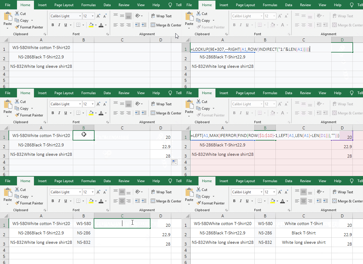
Figure 6
(4) Formula description:
A. The formula for splitting the "number" on the right: =LOOKUP(9E+307,--RIGHT(A1,ROW(INDIRECT("1:"&LEN(A1)))))
(a) The 9E+307 is the maximum value in excel.
(b) LEN(A1) returns the length of the content in A1, the result is 28. INDIRECT("1:"&LEN(A1)) becomes INDIRECT("1:"&28), further calculate, it becomes INDIRECT("1:28"), then returns the reference to the text "1:28", that is, returns $1:$28.
(c) ROW(INDIRECT("1:"&LEN(A1))) becomes ROW($1:$28), then returns the row numbers of 1 to 28 as an array, ie {1,2,3,4,5,6,7,8,9,10,11,12,13,14,15,16,17,18,19,20,21,22,23,24,25,26,27,28}.
(d) --RIGHT(A1,ROW(INDIRECT("1:"&LEN(A1)))) becomes --RIGHT(A1,{1,2,3,4,5,6,7,8,9,10,11,12,13,14,15,16,17,18,19,20,21,22,23,24,25,26,27,28}), when executing,
first, takes 1 from the array, extracts 1 character from the content in A1 with Right function, ie extracts "0";
second, takes 2 from the array, extracts 2 characters from the content in A1 with Right function, ie extracts "20";
the other and so on, finally returns {"0","20","t20",...,"WS-580White cotton T-Shirt20"}.
(e) Formula becomes =LOOKUP(9E+307,--{"0","20","t20",...,"WS-580White cotton T-Shirt20"}), then converts each element of the array to number, the array become {0,20,#VALUE!,...,#VALUE!}, finally lookup the 9E+307 in the array {0,20,#VALUE!,...,#VALUE!}, because it is not found, it returns the maximum value less than or equal to 9E+307, which returns 20.
Hint: splitting the "number" on the right can use the formula: =-LOOKUP(,-RIGHT(A1,ROW(INDIRECT("1:"&LEN(A1))))).
B. The formula for splitting the alphanumeric on the left: =LEFT(A1,MAX(IFERROR(FIND(ROW($1:$10)-1,LEFT(A1,LEN(A1)-LEN(D1))),"")))
(a) ROW($1:$10) returns the array {1,2,3,4,5,6,7,8,9,10}, ROW($1:$10)-1 returns the array {0,1,2,3,4,5,6,7,8,9}.
(b) LEN(A1) returns 28; LEN(D1) returns the number of the values in D1, the result is 2; LEN(A1)-LEN(D1) becomes 28-2, the result is 26; LEFT(A1,LEN(A1)-LEN(D1)) becomes LEFT(A1,26), then extracts 26 characters from left from the content in A1, the result is "WS-580White cotton T-Shirt".
(c) FIND(ROW($1:$10)-1,LEFT(A1,LEN(A1)-LEN(D1))) becomes FIND({0,1,2,3,4,5,6,7,8,9},"WS-580White cotton T-Shirt"), whec executing,
first, takes 0 from the array, lookups 0 in "WS-580White cotton T-Shirt" with Find function, it returns 6;
second, takes 1 from the array, lookups 2 in "WS-580White cotton T-Shirt" with Find function, because 2 is not found, returns the #VALUE!;
the other and so on, finally returns {6,#VALUE!,#VALUE!,#VALUE!,#VALUE!,4,#VALUE!,#VALUE!,5,#VALUE!}.
(d) IFERROR(FIND(ROW($1:$10)-1,LEFT(A1,LEN(A1)-LEN(D1))),"") becomes IFERROR({6,#VALUE!,#VALUE!,#VALUE!,#VALUE!,4,#VALUE!,#VALUE!,5,#VALUE!},""), then checks each element in the array, if it is #VALUE!, returns "", otherwise returns numbers, finally returns {6,"","","","",4,"","",5,""}.
(e) The formula becomes =LEFT("WS-580White cotton T-Shirt",MAX({6,"","","","",4,"","",5,""})), further colulation, returns the maximum 6 in the array; the formula finally becomes =LEFT("WS-580White cotton T-Shirt",6), extracts 6 characters form left from "WS-580White cotton T-Shirt", the result is "WS-580".
C. The formula for splitting the letters in the middle: =SUBSTITUTE(SUBSTITUTE(A1,B1,""),D1,"")
(a) The formula consists of two SubStitute functions nested inside, in which SUBSTITUTE(A1,B1,"") is used to replace the content of B1, that is, replace B1 in A1 with "" (replace "WS-580" with "" in "WS-580White cotton T-Shirt20").
(b)The outer SubStitute is used to replace the content of D1, after SUBSTITUTE (A1, B1, "") replacement, the formula becomes: =SUBSTITUTE("White cotton T-Shirt20",D1,""), replace the text of D1(20) with "", and finally return to "White cotton T-Shirt".
Hint: "" can be omitted "" in the formula =SUBSTITUTE(SUBSTITUTE(A1,B1,""), D1,""), which can be written as follows: =SUBSTITUTE(SUBSTITUTE(A1,B1,), D1,). In addition, splitts the letters in the middle also use the formula: =MID(A1,LEN(B1)+1,LEN(A1)-LEN(B1)-LEN(D1)).
-
Related Reading
- Excel Search function and SearchB usage(13 examples,
- How to move rows,columns,cells,table in excel(there
- Excel left function usage(8 examples, with Sum+Value
- Excel Mid function and Midb usage(6 examples, includ
- How to use Excel Trim function(6 examples, with lead
- How to merge cells in excel(three ways to combine, w
- How to wrap text in excel(with shortcut, automatical
- Excel substitute function usage(8 examples, with mul
- How to use Excel find function(9 examples, include f
- How to wrap text in excel and displays paragraph in