How to use excel Index function, include it and Match,Small,If combination achieve multiple criteria

In Excel, the Index function is used to return an array, or a value or the reference to a value from within a table or range. It is divided into an array form and a reference form; the difference between the two is that the array form can only refer to a contiguous range, the reference form can references to a contiguous range and multiple non-contiguous ranges, and you can also set which range to return.

The Index function is often used in conjunction with functions such as Match, Small, If, and Row. Index and Match combine to return multiple values in the cells at the intersection of row_nums and column_nums, and find the value that satisfy multiple conditions. Index combine Small, If, and Row function can achieve one-to-many lookup and many-to-many lookups that satisfy multiple conditions.

I, Excel Index function syntax

(I) Array form

1. Expression: INDEX(Array, Row_Num, [Column_Num])

2. Description:

A. If both Row_Num and Column_Num are greater than 0, the Index function returns the value in the cell at the intersection of Row_Num and Column_Num; if Column_Num is greater than 0, Row_Num is 0, the entire column is returned; if Row_Num is greater than 0, Column_Num is 0, and the entire row is returned.

B. If you want to return the value as an array, the row should be entered as a horizontal cell range, and the column should be entered as a vertical cell area; for example: {2,3,5;6,9,12}, "2,3,5;" is a row, the row is divided into three columns. In addition, you must press Ctrl + Shift + Enter to return an array.

C. Row_Num and Column_Num must point to the same cell, otherwise a reference error #REF! will be returned; in addition, array formulas cannot be used in Excel Web App.

(II) Reference form

1. Expression: INDEX(Reference, Row_Num, [Column_Num], [Area_Num])

2. Description:

A. If argument Reference refers to a discontinuous range, it must be enclosed in parentheses; for example: (A1:C3, D4:E9).

B. Area_Num is optional. If it is set to 1, it means returning to the first range; if it is set to 2, it returns to the second range; and so on; if Area_Num is omitted, the first range is returned by default.

C. According to the needs of the formula, the Index function returns a reference or a value; for example, the Index function in the formula =SUM(INDEX(D2:E8,3,2)) returns a reference to E4; and the formula=5*INDEX(D2: E8,3,2) Returns the value in the cell E4, as shown in the example below.

D. Except for the above points, the other is the same as the array form.

II, The use examples of Excel Index function array form

(I) Return the cell at the intersection of Row_Num and Column_Num

1. Double-click the cell E9, copy the formula =INDEX(D2:E8,3,2) to E9, press Enter, return to 892; the operation steps are as shown in Figure 1:

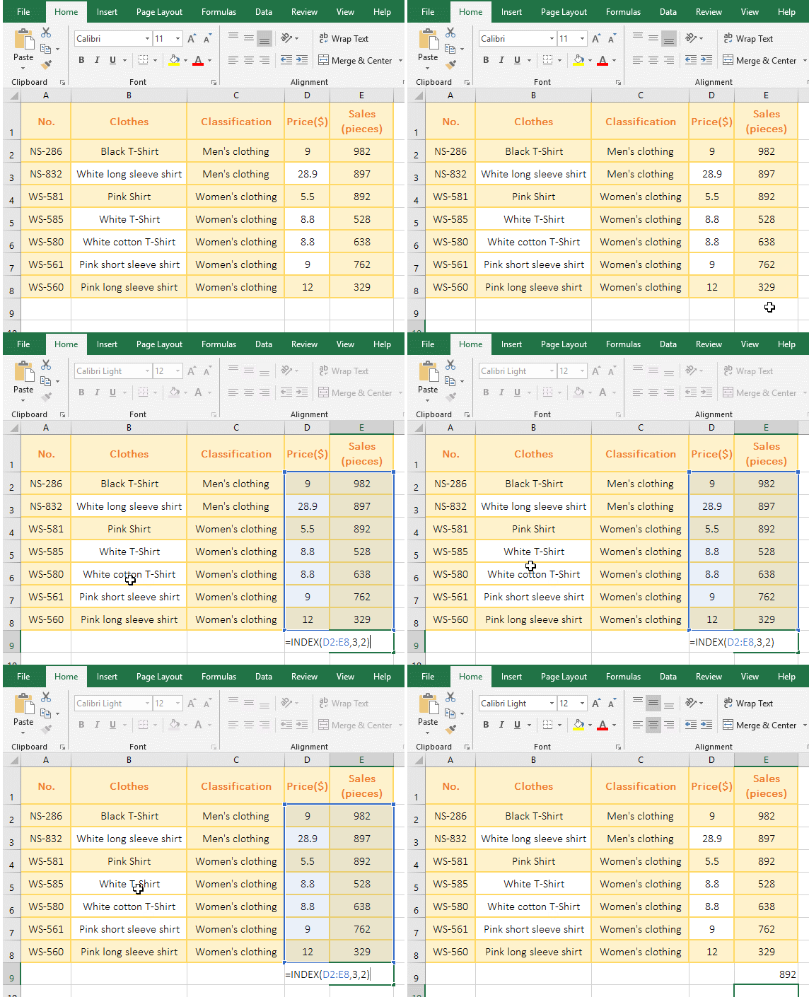
Figure 1

2. D2:E8 is the reference cell range in the formula, because the array form argument Array of the Index function can be either an array or reference to a cell range, the second argument 3 is the return Row_Num, and the third argument 2 is the return Column_Num. Because the returned Row_Num and Column_Num are not 0, so return the value in the cell at the intersection of Row_Num and Column_Num, which is exactly E4; Note: the returned Row_Num and Column_Num start from the selected range.

(II) Argument Array is an array constant

1. Double-click the cell A1, copy the formula =INDEX({3,8,11;4,7,9},2,3) to A1, press Enter, return to 9; the operation steps are as shown in Figure 2:

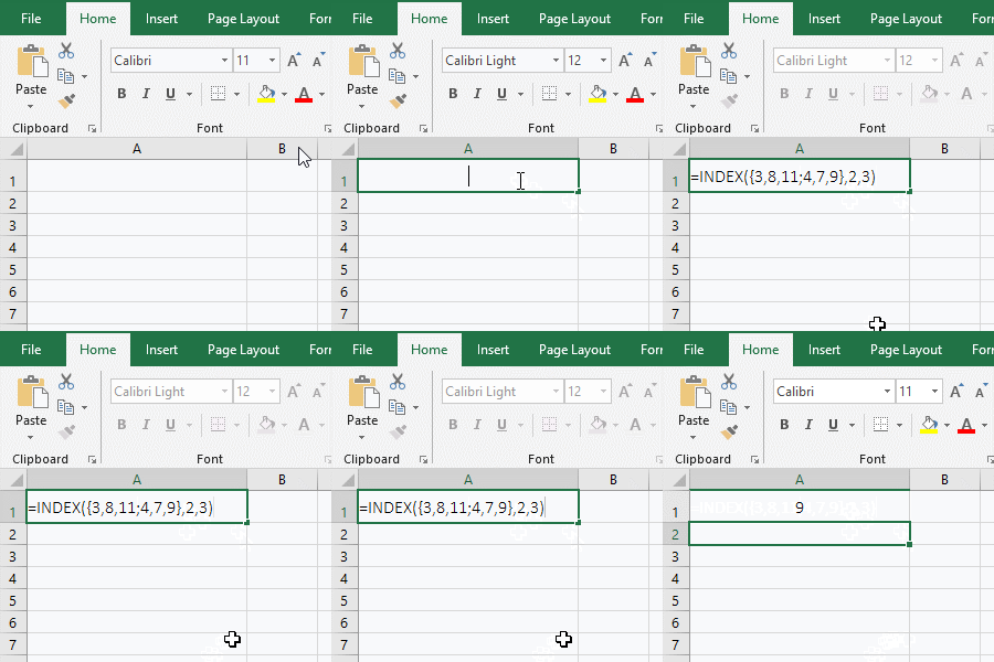
Figure 2

2. {3,8,11;4,7,9} is an array of two rows and three columns in the formula, separated by a semicolon(;) between the rows; the return Row_Num and Column_Num are 2 and 3, that is, return the value in the cell at the intersection of the second row and third column, which is exactly 9.

(III) Return the reference error value #REF!

1. Double-click the cell E9, copy the formula =INDEX(D2:E8,2,3) to E9, press Enter, return the reference error value #REF!; The operation steps are as shown in Figure 3:

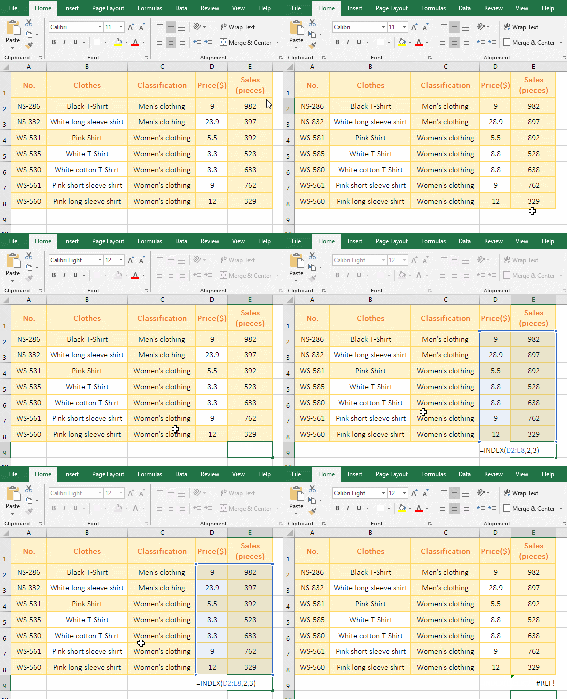
Figure 3

2. The formula reference range D2:E8 only two rows and two columns, and the return Column_Num is 3, which refers to the column does not exist, so the reference error is returned.

III, The use examples of Excel Index function reference form

(I) Instances that reference multiple discontinuous Areas

1. Double-click the cell B10, copy the formula =INDEX((B2:C4,D6:E9),2,1,2) to B10, press Enter, return to 892; the operation steps are as shown in Figure 4:

Figure 4

2. The reference (B2:C4, D6:E9) in the formula is two non-contiguous Areas, so it should be enclosed in parentheses; returned Area_Num is 2, that is, return the second Area, the Row_Num and Column_Num that has been returned are 2 and 1, respectively, which returns the value in the cell at the intersection the second row and the first column in D6:E9, which is D7.

(II) Omit the argument Area_Num

1. Double-click the cell B10, copy the formula =INDEX((B2:C4,D6:E9),2,1) to B10, press Enter, return to 215; double-click B10 again, remove the ", D6:E9" and one Left bracket"(" , the formula becomes =INDEX(B2:C4,2,1), press Enter, still return to 215; the operation steps, as shown in Figure 5:

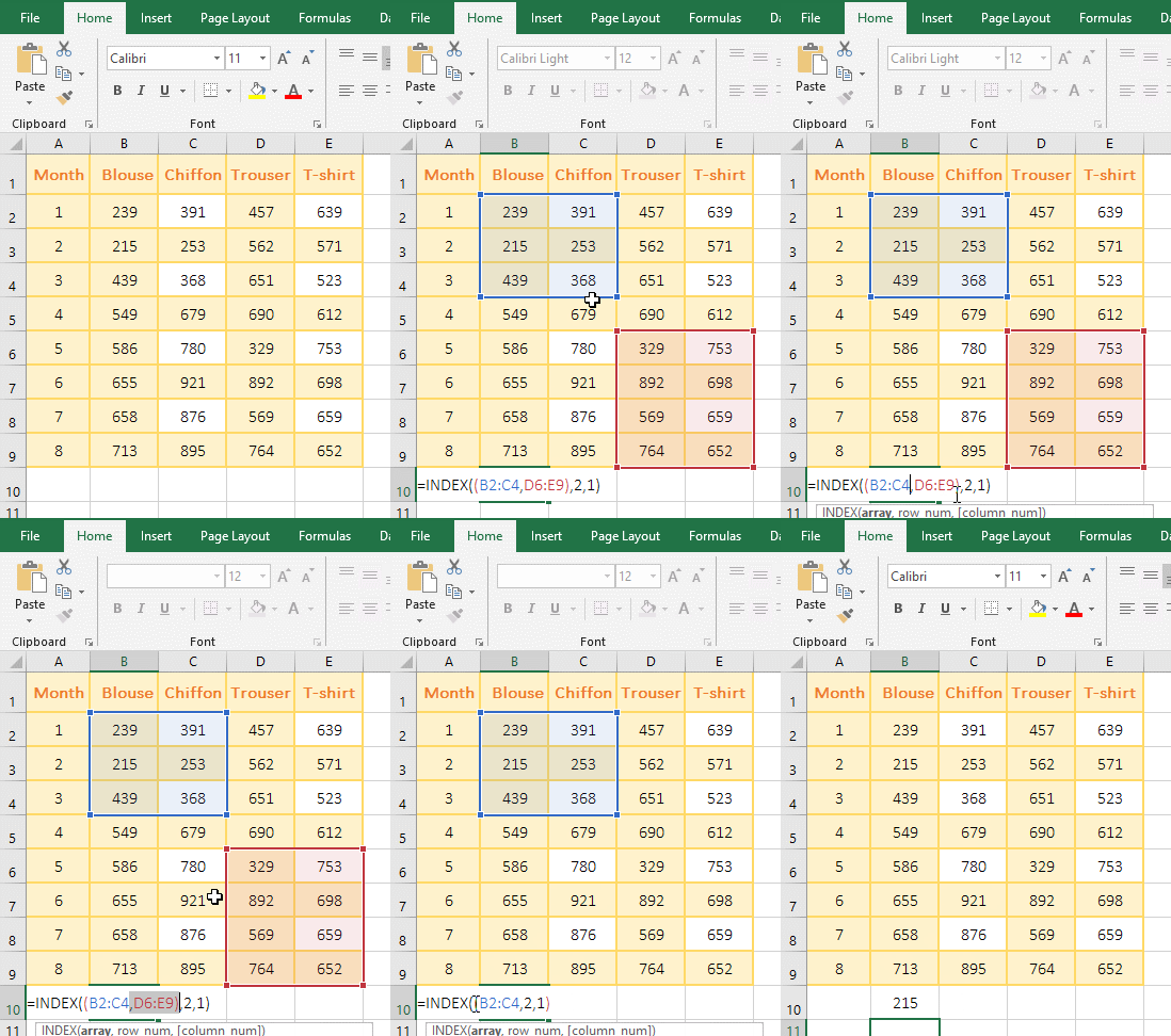
Figure 5

2. The argument Area_Num is omitted in the formula =INDEX((B2:C4,D6:E9),2,1), the first area B2:C4 is selected by default, and the value in the cell(B3) at the intersection of the second row and the first column is returned; the formula =INDEX(B2:C4,2,1) is the same as the array form.

(III) Return the reference to cell

1. Double-click the cell E9, copy the formula =SUM(INDEX(D2:E8,3,2)) to E9, press Enter, return to 892; press and hold Alt, press M, V one time, and open the "Evaluate Formula "Window, click "Evaluate", the formula becomes SUM($E$4), indicating that the Index function returns a reference to E4; the operation process steps, as shown in Figure 6:

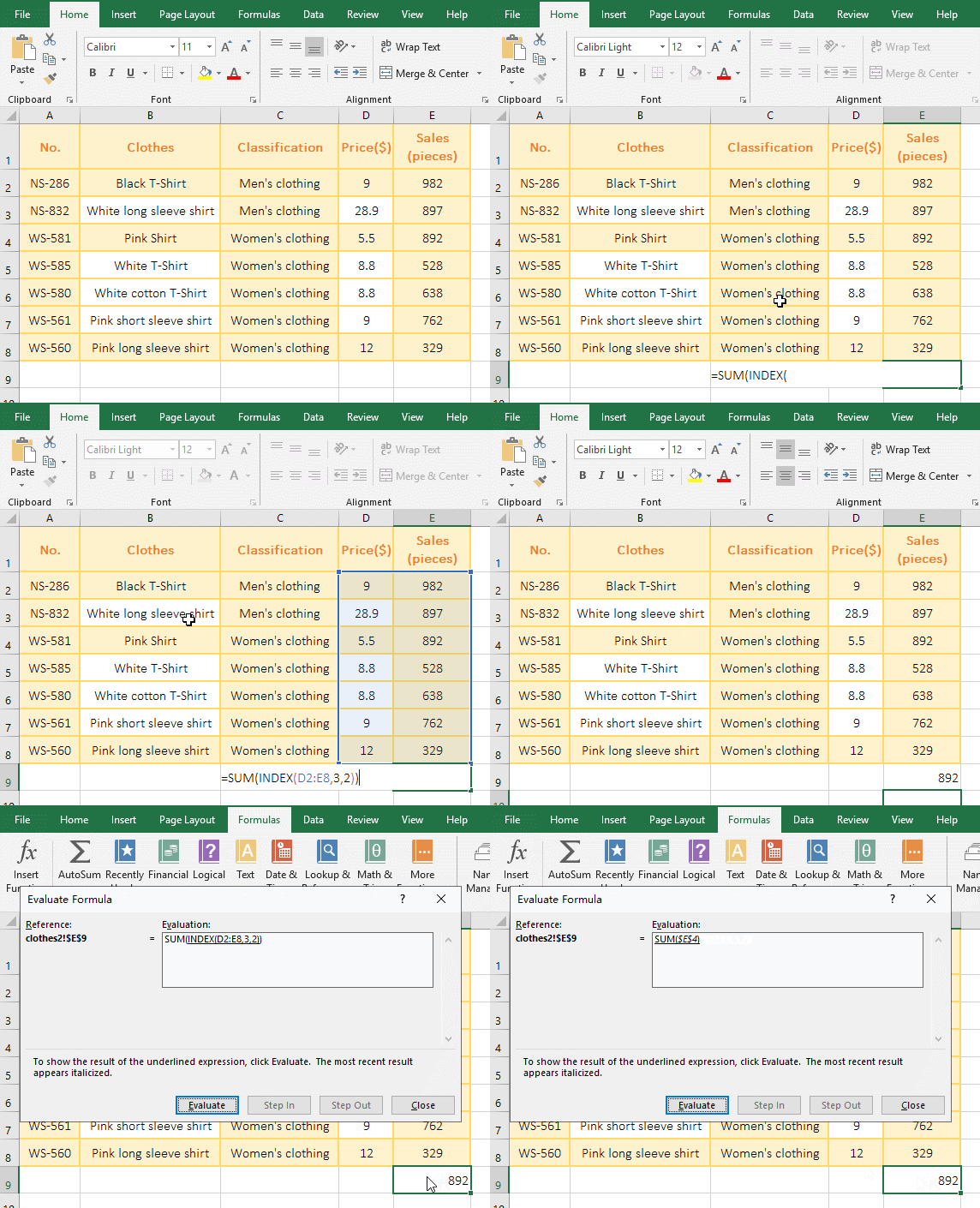
Figure 6

2. SUM($E$4) means summing E4, and $E$4 means absolute reference to cell E4.

(IV) Return a value in the reference cell

1. Double-click the cell E9, copy the formula =5*INDEX(D2:E8,3,2) to E9, press Enter, return to 4460; hold down Alt, press M, V one time, and open "Evaluate Formula" Window, press Enter to "Evaluate", the formula becomes 5 * 892, indicating that the Index function returns the value in the reference cell; the operation process steps, as shown in Figure 7:

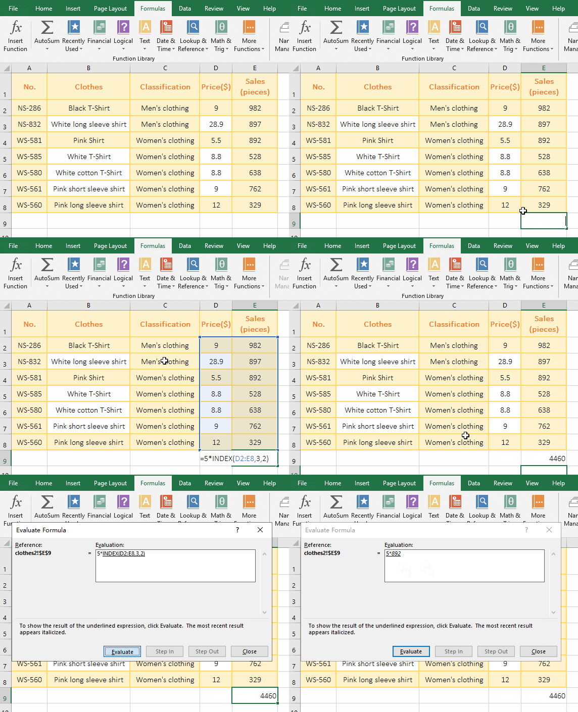
Figure 7

2. From the above two examples, the Index function can return the value in the cell or references to cell according to the actual needs of the formula.

(V) Index + Sum function combination returns the entire row or entire column

1. Copy the formula =SUM(INDEX(B2:E9,2,0)) to the cell E10 and press Enter to return to 1601. Hold down Alt and press M and V one time to open the "Evaluate Formula" window. Press Enter to "evaluate" and the formula changes to SUM($B$3:$E$3), B3:E3 is the second row of the selected area. Double-click E10, change the formula to =SUM(INDEX(B2:E9,0,3)), press Enter, return to 4914, open the "Evaluate Formula" window in the same way, press Enter, the formula changes to SUM($D$2:$D$9), D2:D9 is the third column of the selected area; the operational steps are shown in Figure 8:

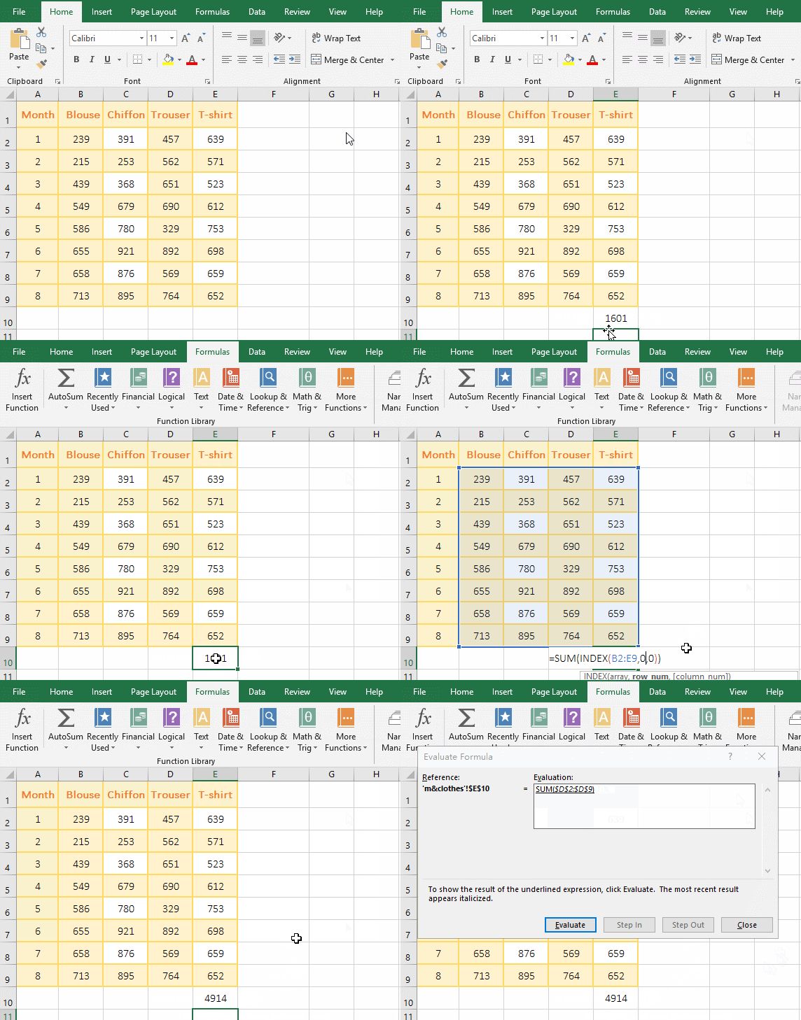
Figure 8

2. The Index function returns the entire row or entire column is usually returned according to the formula, only a single Index formula can not be returned.

IV, The extended application of Excel Index function

(I) Index + Match function combination returns multiple values in the cells at the intersection of the Row_Nums and Column_Nums(index match formula in excel)

1. If you want to return the sales of various types of clothing every month. Double-click the cell B12 and copy the formula =INDEX($A$1:$E$9, MATCH($A12,$A$1:$A$9,), MATCH(B$11,$A$1:$E$1,)) to B12, press Enter, return 239; Select B12, move the mouse to the cell fill handle in the lower right corner of B2, after the mouse turns into the bold balck cross, hold down the left button, drag to the right, drag to E12, then the cell will return the corresponding sales; Move the mouse to the cell fill handle in the lower right corner of E12, and drag down to return the clothing sales of "March and June"; the operation steps are as shown in Figure 9:

Figure 9

2. Formula =INDEX($A$1:$E$9, MATCH($A12,$A$1:$A$9,), MATCH(B$11,$A$1:$E$1,)) description:

A. $A$1 is an absolute reference to the row and column, drag down, A1 will not become A2, A3, ...; drag to the right, A1 will not become B1, C1, .... $A$1:$A$9 returns the data from A1 to A9 as an array.

B. MATCH($A12, $A$1:$A$9,) Find A12(January) in A1 to A9, return 2 that is index of A12 in A1:A9; the Match function omits the last argument, the default is 1 , which returns a maximum value less than or equal to the lookup value.

C. MATCH(B$11, $A$1:$E$1,) Look for B11(Blouse) in A1 to E1, and the return index is also 2.

D. The formula becomes =INDEX($A$1:$E$9,2,2), which returns the value in the cell B2 at the intersection of the second row and the second column in A1:E9, which is 239.

Tip: If the data you dragged is the same, press Ctrl + C to save.

(II) Excel index match multiple criteria

1. If you want to find the name of the clothing whose "Classification" equal "Men's clothing" and price equal 80. Double-click the cell C11 and copy the formula =INDEX(B2:D8,MATCH(A11&B11,C2:C8&D2:D8,),1) to C11, press Ctrl + Shift + Enter to return to the "Black T-Shirt"; the process steps, as shown in Figure 10:

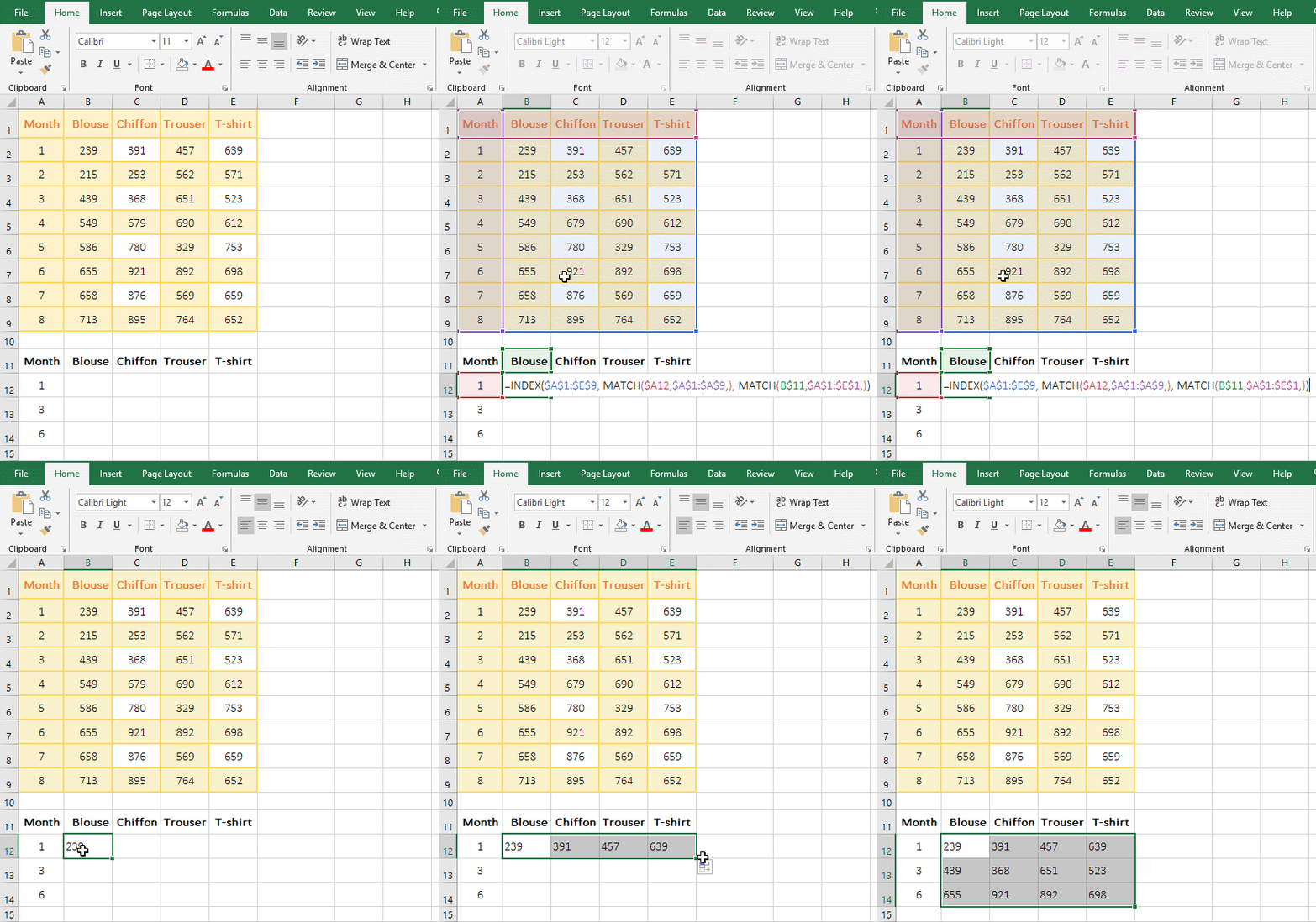
Figure 10

2. Formula =INDEX(B2:D8,MATCH(A11&B11,C2:C8&D2:D8,),1) description:

A. The formula is an array formula, so press Ctrl + Shift + Enter.

B. A11&B11 means that connects A11 and B11, and C2:C8&D2:D8 means that connects the values corresponding to each row of C2:C8 and D2:D8, such as C2&D2, C3&D3.

C. Then MATCH (A11&B11,C2:C8&D2:D8,) becomes MATCH ("Men's clothing9", {"Men's clothing9"; "Men's clothing28.9"; "Women's clothing5.5"; "Women's clothing8.8"; "Women's clothing8.8"; "Women's clothing9"; "Women's clothing12"},), then look for "Men's clothing9" in the array, find it and return it to index 6 in the array.

D. The formula becomes =INDEX(B2:D8,6,1), and finally the value in the cell at the intersection of the first column and the sixth row is returned in B2:D8, that is, the "Black T-Shirt" in B7.

(III) Index + Small + IF + Row function combination to achieve one-to-many search

1. If you want to find the names and positions of all employees in the "Finance". Double-click the cell F2 and copy the formula =IFERROR(INDEX(A:A,SMALL(IF(B$2:B$9=$E$2,ROW($2:$9),4^8),ROW(A1))),"") to F2, press Ctrl + Shift + Enter to return to "Shiery"; select F2, drag down, return to the other employee name of "Finance"; double click G2, put the above formula Copy to G2, and change A:A in the formula to C:C, press Ctrl + Shift + Enter to return to "Employees", and also use the method of dragging down to return to other employees; the operation steps are as shown in Figure 11:

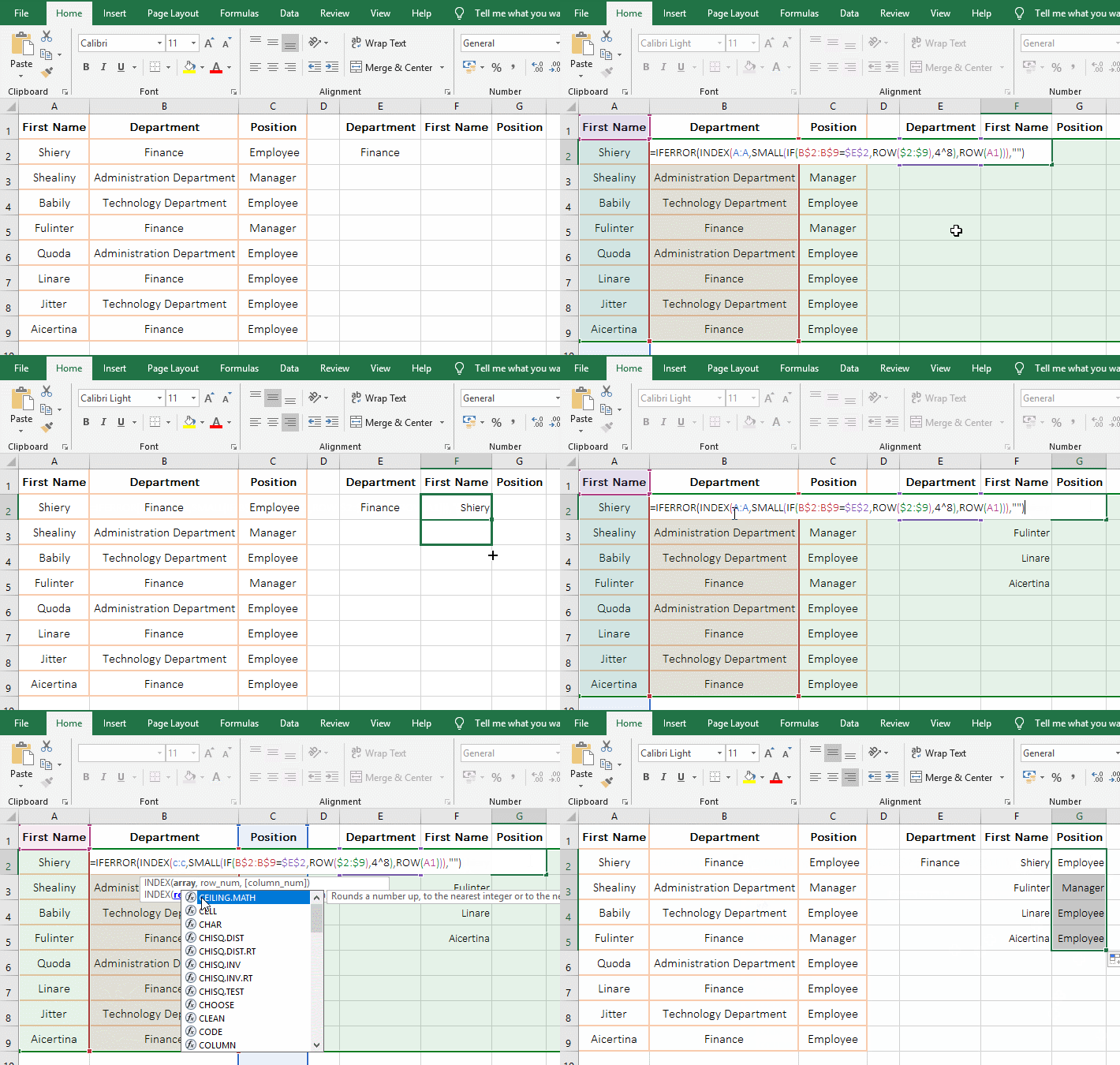
Figure 11

2. The formula =IFERROR(INDEX(A:A,SMALL(IF(B$2:B$9=$E$2,ROW($2:$9),4^8),ROW(A1))),"") description:

A. B$2:B$9 returns the elements in B2 to B9 as an array, ie {"Finance"; "Administration Department"; "Technology Department"; "Finance"; "Administration Department"; "Finance"; "Technology Department";"Finance"};$E$2 is "Finance"; then B$2:B$8=$E$2 becomes {"Finance"; "Administration Department"; "Technology Department"; "Finance"; "Administration Department"; "Finance"; "Technology Department";"Finance"}="Finance", then compare each element in the array with "Finance", return True if equal, otherwise return False, and finally return {TRUE;FALSE;FALSE;TRUE;FALSE;TRUE;FALSE;TRUE}.

B. ROW($2:$89) returns the value between 2 and 9 as an array, ie {2;3;4;5;6;7;8;9}; 4^8 is the 8 power of 4, the result is 65536 (the maximum supported by Excel).

C. Then IF(B$2:B$9=$E$2,ROW($2:$89),4^8) becomes IF({TRUE;FALSE;FALSE;TRUE;FALSE;TRUE;FALSE;TRUE},{2;3;4;5;6;7;8;9},65536), then, the first element TRUE is taken from the conditional array, since it is true, the value that is the second argument of If is returned, ie the element 2 that is the element of the array {2;3;4;5;6;7;8;9} corresponding to the conditional array is returned; the second time to take the second element FALSE from the conditional array, because it is false, so return the third argument of If, that is, return 65536; finally return {2;65536;65536;5;65536;7;65536;9}.

D. ROW(A1) returns the Row_Num 1 of A1; then SMALL(IF(B$2:B$9=$E$2,ROW($2:$9),4^8),ROW(A1) becomes SMALL({2;65536;65536;5;65536;7;65536;9},1), then, use Small function to find the first small value in the array, which is 2.

E. The formula becomes =IFERROR(INDEX(A:A,2),""), A:A means to refer to column A, and finally returns the value of the second row in column A, which returns the value(Shiery) in A2. "IfError is used for error handling. If INDEX(A:A,2) returns an error, it returns null, otherwise it returns the return value of INDEX(A:A,2).

Tip: If you want to find employees in other departments, change the "Finance" in E2 to another department and press Enter. If there is no change, just press Ctrl + S to save. If you want to display all the returned values to one row, for example, to display the "Finance" employee to a row, just change ROW(A1) in the formula to COLUMN(A1), then the formula becomes =IFERROR(INDEX(A:A,SMALL(IF(B$2:B$9=$E$2,ROW($2:$9),4^8),COLUMN(A1))),""), drag to the right.

(IV) Index + Small + IF + Row function combination to achieve multi-condition and many-to-many lookup

1. If you want to lookup the clothing name whose "Classification" equal "Women's clothing" and price equal 80. Double-click on the cell C11 and Copy the formula =IFERROR(INDEX(B:B,SMALL(IF((C$2:C$8=$A$11)*(D$2:D$8=$B$11),ROW($2:$8),4^8),ROW(A1))),"") to C11, press Ctrl + Shift + Enter to return to "White T-Shirt"; use the method of dragging down to return other eligible clothing names; the steps are as shown in Figure 12:

Figure 12

2. The formula is the same as the above Index + Small + IF + Row function combination formula, the only difference is that the condition of If consists of multiple expressions, each expression is connected by an asterisk (*), indicating "AND" relationship, which is to satisfy multiple conditions at the same time.