 Office > Excel > Excel 2019 > Content
How to use Excel small function and it and index, match combine to screen non-duplicate in formula
The Excel Small function is used to return a specified value in an array or a reference cell sorted from small to large, such as the first minimum, the second minimum, and so on. It has only two arguments, one is Array and the other is k, k cannot be less than or equal to 0 and cannot be greater than the total number of array elements, otherwise an error is returned.
Excel Small functions is often combined with Index, IF, Match, and Row functions to achieve one-to-many lookups on the one hand and filter duplicate values on the other hand. These two aspects are widely used. Let's first study the basic usage of the Small function, and then study the extended application combined with each function.
I, Excel Small function syntax
1. Expression: SMALL(Array, k)
2. Description:
If argument Array is empty and k is less than or equal to 0 or k is greater than the number of values in the Array, Small function returns the numeric error value #NUM!.
II, The examples of Excel Small function
(I) Example with duplicate values in Array
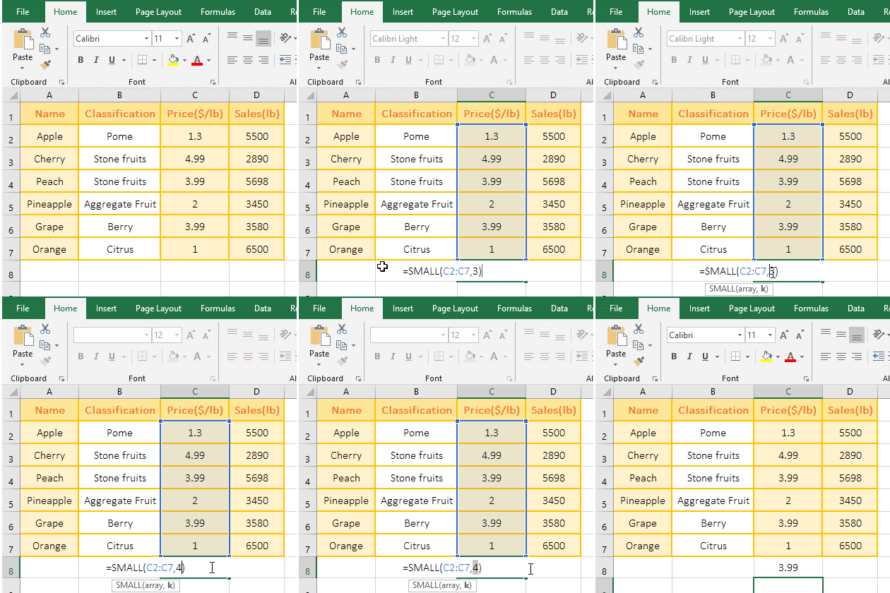
1. Double-click the cell C8, copy the formula =SMALL(C2:C7,3), paste it in C8, press Enter, return to the 3rd minimum 2; double-click C8, change 3 to 4, press Enter, return to the 4th minimum 3.99; double-click C8 again, change 4 to 5, press Enter, return to the 5th minimum 3.99; the operation steps, as shown in Figure 1:

Figure 1
2. Small formula description:
A. C2:C7 is the Array, 3 is the return position(k) in the formula =SMALL(C2:C7,3); the formula means to return the 3rd smallest number in C2 to C7, C2:C7 is not sorted.
B. Formula =SMALL(C2:C7,4) and =SMALL(C2:C7,5) both return 3.99, indicating that the Small function arranges the duplicate values to two different positions, such as 3.99 in the example, one rank 4th, the other rank 5th.
(II) Example of return the numeric error value #NUM!
1. Double-click the cell D8, copy the formula =SMALL(D2:D7,0) to D8, press Enter, return the numeric error value #NUM!; double-click D8, change 0 to 7, press Enter, and return #NUM!; operation process steps, as shown in Figure 2:

Figure 2
2. Formula =SMALL(D2:D7,0) Returns the 0th minimum value in D2:D7. Since argument K must be greater than 0, return #NUM! Error; the formula =SMALL(D2:D7,7) returns the 7th minimum value, since there are only 6 values in D2:D7, and argument K must be less than or equal to 6, so return #NUM! error.
III, The Excel Small function extension use case
(I) Excel index small IF Row function combination to achieve one-to-many search
The detailed analysis of the Index + Small + IF + Row combination has been introduced in the article "How to use excel Index function, include it and Match,Small,If combination achieve multiple criteria". Click on the title of the article in double quotes.
(II) Excel index match small IF Row function combination to achieve screening non-duplicate value(unique value)
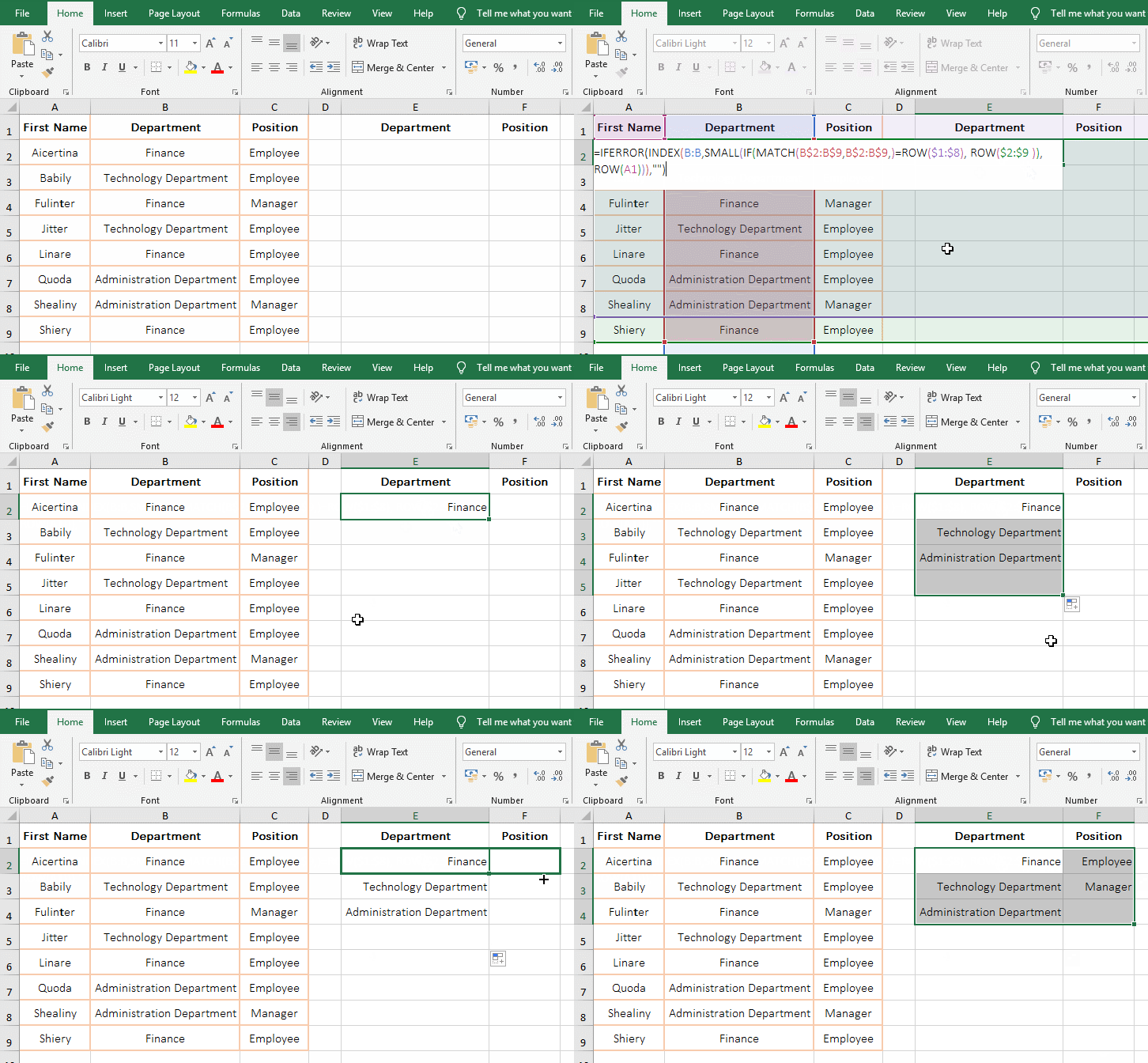
1. Double-click the cell E2, copy the formula =IFERROR(INDEX(B:B,SMALL(IF(MATCH(B$2:B$9,B$2:B$9,)=ROW($1:$8), ROW($2:$9)), ROW(A1))),"") to E2, press Ctrl + Shift + Enter to return to "Finance"; move the mouse to the cell fill handle in the lower right corner of E2, after the mouse becomes the bold black plus(+), hold down the left button and drag down until the empty cell appears, filter out all the duplicate values of the "Department" in column B; select E2, drag to the right, and return to the first value("Employee") that is non-duplicate in column C, drag it down, and drag it all the way to the empty cell, then return all the non-duplicate values of column C; the operation steps, as shown in Figure 3:

Figure 3
2. Formula =IFERROR(INDEX(B:B,SMALL(IF(MATCH(B$2:B$9,B$2:B$9,)=ROW($1:$8), ROW($2:$9)), ROW(A1))),"") description:
A. The $ in B$2 represents the absolute reference to the row, when dragging down, 2 does not become 3, 4, etc.; B$2:B$9 returns all the departments in B2 to B9 as an array, ie {"Finance"; "Technology Department"; "Finance"; "Technology Department"; "Finance"; "Administration Department"; "Administration Department";"Finance"}.
B. When MATCH(B$2:B$9, B$2:B$9,) executed, the first time takes out B2(ie "Finance") from B2:B9, then return to the position(ie 1) of "Finance" in B2:B9; Second B3(ie "Technology Department") is taken out, returns to position 2 in B2:B9; the others and so on, and finally returns the array {1;2;1;2;1;6;6;1}; The main thing is that the same value returns the same position.
C. $1:$8 is used to return an array of 1 to 8, ie {1;2;3;4;5;6;7;8}; ROW($1:$8) is used to return the row number from 1 to 8, ie {1;2;3;4;5;6;7;8}. ROW($2:$9) is used to return the row number from 2 to 9, ie {2;3;4;5;6;7;8;9}.
D. Then IF(MATCH(B$2:B$9, B$2:B$9,)=ROW($1:$8), ROW($2:$9)) becomes IF({1;2;1;2;1;6;6;1}={1;2;3;4;5;6;7;8},{2;3;4;5;6;7;8;9}), then take the first element 1 from the array on the left of =, then take the first element 1 from the array on the right of =, they are equal, so return True; the second time take the second element 2 from the left array of = and take the second element 2 from the right array of =, they are also equal, so they also return True; others and so on, and finally return the array {TRUE; TRUE; FALSE; FALSE; FALSE; TRUE; FALSE; FALSE}. This step is mainly to filter out duplicate values, leaving only the first department of the duplicate department, it will be leave for True.
E. Then IF({1;2;1;2;1;6;6;1}={1;2;3;4;5;6;7;8},{2;3;4;5;6;7;8;9}) becomes IF({TRUE;TRUE;FALSE;FALSE;FALSE;TRUE;FALSE;FALSE}, {2;3;4;5;6;7;8;9}), and then takes the first element TRUE from the array of condition, which is true, returns the corresponding element 2 of the second argument of If(ie return 2 in {2;3;4;5;6;7;8;9}); the second time takes the second element TRUE, returns the corresponding element 3 in {2;3;4;5;6;7;8;9}; the third time takes FALSE, it is false, so it returns the third argument of If, because it is omitted here, it returns FALSE by default; finally it returns {2;3;FALSE;FALSE;FALSE;7;FALSE;FALSE}.
F. ROW(A1) is used to return the row number 1 of A1; then SMALL(IF(MATCH(B$2:B$9,B$2:B$9,)=ROW($1:$8), ROW($2:$9)), ROW(A1)) becomes SMALL({2;3;FALSE;FALSE;FALSE;7;FALSE;FALSE},1), and then returns the first minimum value 2 in the array.
G. The formula becomes =IFERROR(INDEX(B:B,2),""), B:B means to refer to column B; then use the Index function to return the value of the second row of column B "Finance". IfError is an error judgment function, it has been introduced several times in the previous chapter.
3. Formula =IFERROR(INDEX(B:B,SMALL(IF(MATCH(B$2:B$9,B$2:B$9,)=ROW($1:$8), ROW($2:$9)), ROW(A1))),"") has two ways to write:
=IFERROR(INDEX(B:B,SMALL(IF(MATCH(B$2:B$9,B$2:B$9,)=ROW(B$1:B$8), ROW(B$2:B$9)), ROW( A1))), "")
=IFERROR(INDEX(B:B,SMALL(IF(MATCH(B$2:B$9,B$2:B$9,)=ROW(B$2:B$9)-1, ROW(B$2:B$9)), ROW(A1))),"")
-
Related Reading
- Excel Search function and SearchB usage(13 examples,
- Excel lookup function usage(Multiple conditional and
- 8 examples of Excel Match function, include it and S
- How to use offset function in excel, include it and
- VLookUp in excel introduces step by step(10 examples
- Excel If function examples, include if statement nes
- How to use Excel address function(7 examples, with I
- How to find duplicate values in excel using vlookup(
- Excel SumIf function with ?/*, Average and array mul
- How to use hlookup in excel(7 hlookup example, combi
- How to use excel Index function, include it and Matc
- Vlookup with if statement(use if/if{0,1} combination