How to use offset function in excel, include it and Sum, Match, CountIf combination in formula

The OffSet function is used to return a reference to a range that is a specified number of rows and columns from a cell or range of cells in excel. The range can be up or down, right or left the base cell, depending on the positive and negative of arguments Rows and Cols of the OffSet function; the size of the referenced range is based on the arguments Height and Width.

The OffSet function is often used in combination with Sum, Match, CountIf, If, Or Row, etc., for example, Sum + OffSet + Match + CountA function combination to achieve dynamic range summation, OffSet + Int + Row function combination to achieve a repeat multiple, CountIf + OffSet + Match + CountIf function combination to achieve segmentation statistics.

I, OffSet function in excel syntax

1. Expression: OFFSET(Reference, Rows, Cols, [Height], [Width])

2. Description:

A. Reference must be a reference to a cell or range of adjacent cells, otherwise the value error #VALUE! will be returned; the return cell is referenced to Reference.

B. Rows refers to the number of rows up or down from the upper-left of Reference. For example, Reference is B3, if Row is 2, it means 2 rows under B3. If Row is -2, it means 2 rows on B3. That is, when Row is a positive number, it refers to the bottom of the reference cell; when Row is a negative number, it refers to the top of the reference cell.

C. Cols refers to the number of columns from left to right in the upper-left of the Reference. For example, Reference is B3; if Cols is 1, it means 1 column to the right of B3 (ie, column C); if Cols -1, it means 1 column to the left of B3 (ie column A). That is, Cols is positive and refers to the right side of the reference cell; Cols is negative, which refers to the left side of the reference cell.

D. Height and Width must be positive; if Height or Width is omitted, they are the same as Reference by default.

E. If Rows and Cols are beyond the edge of the table, the OffSet function will return the reference error value #REF!.

II, The examples of OffSet function in excel

(I) Rows or Cols equal 0

1. Double-click cell A10, copy the formula =OFFSET(A1,3,) to A10, press Enter, return to "Fulinter"; double-click A10 again, change the formula to =OFFSET(A1,,2), press Enter , return to "Position"; the operation process steps, as shown in Figure 1:

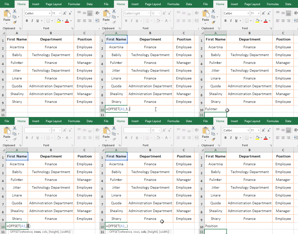
Figure 1

2. Formula description:

A. A1 is the reference cell, 3 is the number of rows from A1, Cols is omitted, the default is 0; Height and Width are omitted, the default is the height and width of A1 in the formula = OFFSET (A1,3,). The meaning of the formula is: return the cell reference of the 3 rows and 0 columns under A1, that is, return to the "Fulinter" in A4.

B. Formula =OFFSET(A1,,2) Omit the Rows, the default is 0; the omitted Height and Width, their values are the same as above; the formula means: return the cell reference C1 of 0 row and 2 column to right of A1, that is, return "Position".

(II) Returning the upper and lower reference of the specified number of rows from the upper-left of the reference cell

1. Double-click cell A8, copy the formula =OFFSET(A2:B3,1,1,1,1) to A8, press Enter, return to "Stone fruits"; double-click A8 again, and set the second argument of OffSet 1 change to -1, press Enter, return to "Classification"; the operation process steps, as shown in Figure 2:

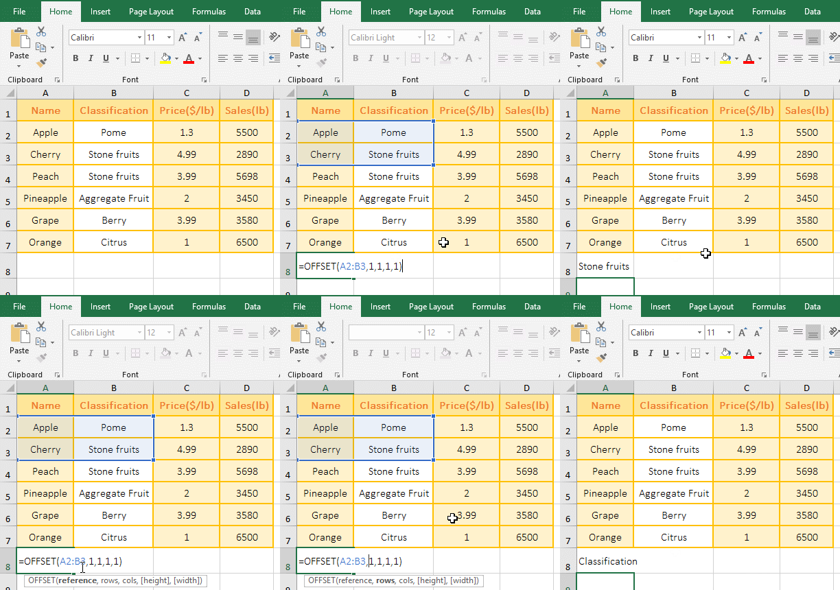
Figure 2

2. A2:B3 is the reference range in the formula =OFFSET(A2:B3,1,1,1,1), meaning: return the reference to the cell 1 row under the upper-left cell of A2:B3(ie A2) and 1 column to right of A2 with height and width to 1, that is, returns the "Stone fruits" in B3. After changing the second argument to -1, it returns a reference to the cell with 1 row above the upper-left cell(ie B1) of A2:B3 and 1 column to right of B1 and height and width to 1, which returns the "classification" in B1.

(III) Return the left and right reference of the specified number of columns from the upper-left of the base cell

1. Double-click cell C10, copy the formula =OFFSET(C4:D5,3,2,1,1) to C10, press Enter, return to 133.13; double-click C10 again, change 2 to -2, press Enter, Return to 6; the process steps, as shown in Figure 3:

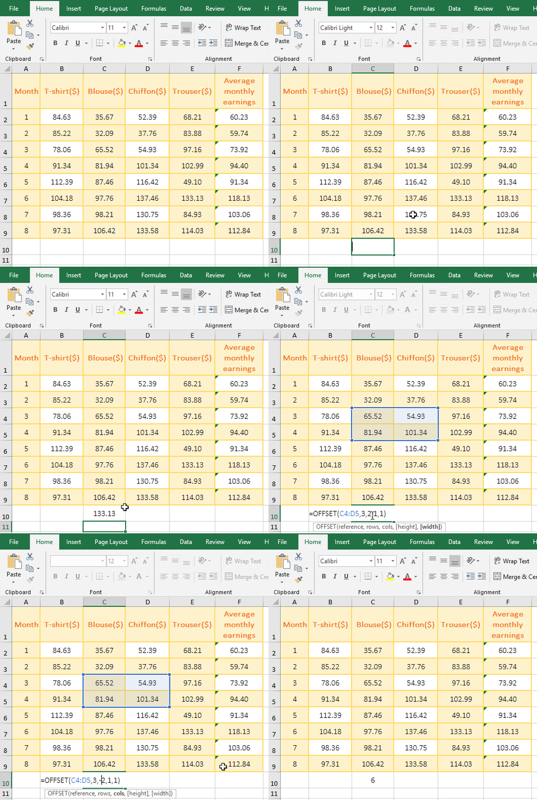
Figure 3

2. C4:D5 is the reference cell range in the formula =OFFSET(C4:D5,3,2,1,1), meaning: return the reference to the cell 3 rows under the upper-left cell(ie C4) of C4:D5 and 2 Columns to  right of C4 with height and width to 1,that is, returns to 133.13 in E7. When 2 is changed to -2, it returns the reference to the cell 3 rows under C4 and 2 columns to left of C4, which returns 6 in A7.

(IV) Return multi-cell reference

1. Double-click cell A8, copy the formula =OFFSET(A2:B3,2,2) to A8, press Enter, return the value error #VALUE!; double-click A8 again, add the argument Height and Width 1 after the formula, press Enter, return 3.99; double-click A8, change the latter two 1 to 2, press Ctrl + Shift + Enter, also return 3.99; the operation steps, as shown in Figure 4:

Figure 4

2. The formula =OFFSET(A2:B3,2,2) is the same as =OFFSET(A2:B3,2,2,2,2), because omits the height and width, they are the same as A2:B3 by default. When you press Enter, they return the wrong value #VALUE!, and press Ctrl + Shift + Enter, but can return 3.99, because returns an array, this is usually used in combination with other functions, as shown in the examples below. Formula =OFFSET(A2:B3,2,2,1,1) Press Enter to return 5 because only one cell is returned.

(V) Return #REF! error

1. Double-click cell A9, copy the formula =OFFSET(A2:B3,-2,2,1,1) to A9, press Enter, return the reference error #REF!; The operation steps are as shown in Figure 5:

Figure 5

2.  -2 indicates the two rows above A2 in the formula =OFFSET(A2:B3,-2,2,1,1), and there is only one row on A2, so the reference error is returned.

III, The extended use case of OffSet function in excel

(I) Excel Offset Match function combination

Detailed analysis of the OffSet + Match function combination has been introduced in the article "8 examples of Excel Match function, include it and Sum, OffSet, Indirect combination to extract data", view please Click on the title of the article in double quotes.

(II) Excel offset dynamic range: Sum + OffSet + Match + CountA function combination to achieve dynamic summation

1. If you want to subtotal the sum of all kinds of clothing sales in any month. Double-click cell B12, copy the formula =SUM(OFFSET(A1,MATCH(A12,A2:A9,),1,1,4)) to B12, press Enter, and return to 1601 that is the sum of the sales of various types of clothing in February. ; double-click B14, copy the formula =SUM(OFFSET(A$1,MATCH(A14,A$2:A$9,),1,1,4)) to B14, press Enter, return to 1726; select B14, move the mouse to the cell fill handle in the lower right corner of B14, after the mouse becomes the bold black plus, hold down the left button and drag down to return the sum of the sales of various types of clothing in "April and July"; the operational process steps, as shown in Figure 6:

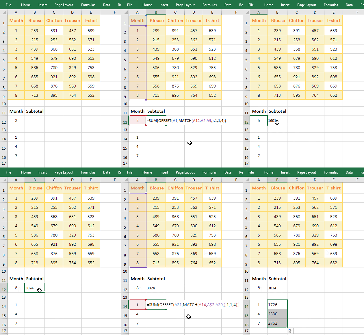
Figure 6

2. Formula description:

The two formulas are the same, except when the latter formula is pulled down, the rows in A1, A2, and A9 are added $ to become absolute references. Below is only one example of the next formula =SUM(OFFSET(A$1,MATCH(A14,A$2:A$9,),1,1,4)).

A. A$2:A$9 returns all the months in A2 to A9 as an array. Drag down, A2 and A9 will not be automatically added 1, such as A2 does not become A3, A4, etc.

B. MATCH(A14,A$2:A$9,) is used to return the position 1 of A14 (ie 1) in A2 to A9; the Match function omits the last argument, and the default is 0 to indicate exact match.

C. Then OFFSET(A$1,MATCH(A14,A$2:A$9,),1,1,4) becomes OFFSET(A$1,1,1,1,4), then returns to the reference to cells 1 row under A1 and 1 column to right of A1 with height to 1, and width to 4, returns B2:E2.

D. The formula becomes =SUM(B2:E2), and finally B2:E2 is summed, so 1726 is returned.

Hint: If there are more columns, the last argument 4 in the formula can be replaced by CountA(B$1:E$1) or COUNTA($1:$1)-1. That is, if the CountA function is used to count the number of columns, the formula becomes=SUM(OFFSET(A$1,MATCH(A14,A$2:A$9,),1,1,CountA(B$1:E$1))). $1:$1 means to reference first row.

3. If you want to dynamically return the sum of any column, apply this formula =SUM(OFFSET(A$1,1,MATCH(A12,B$1:E$1,), COUNTA(A$2:A$9),1)), demo As shown in Figure 7:

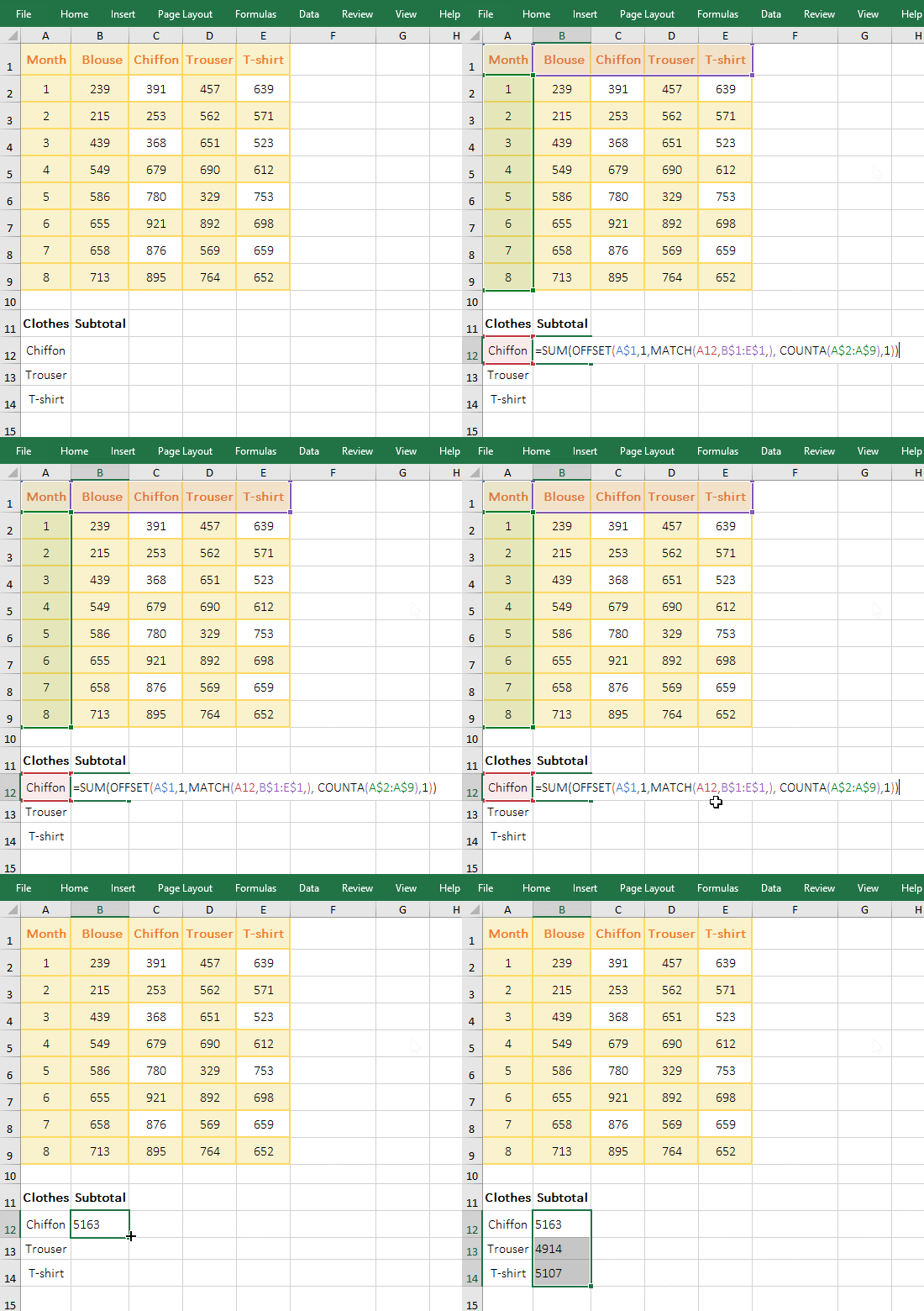
Figure 7

(III) OffSet + Int + Row function combination implementation to make a repeat multiple

1. If you want to repeat each fruit name in column A three. Double-click cell A9, copy the formula =OFFSET(A$2,INT((ROW(A1)-1)/3),0) to A9, press Enter, return to "Apple"; select A9, drag down repeats the remaining names three times; the operation steps are as shown in Figure 8:

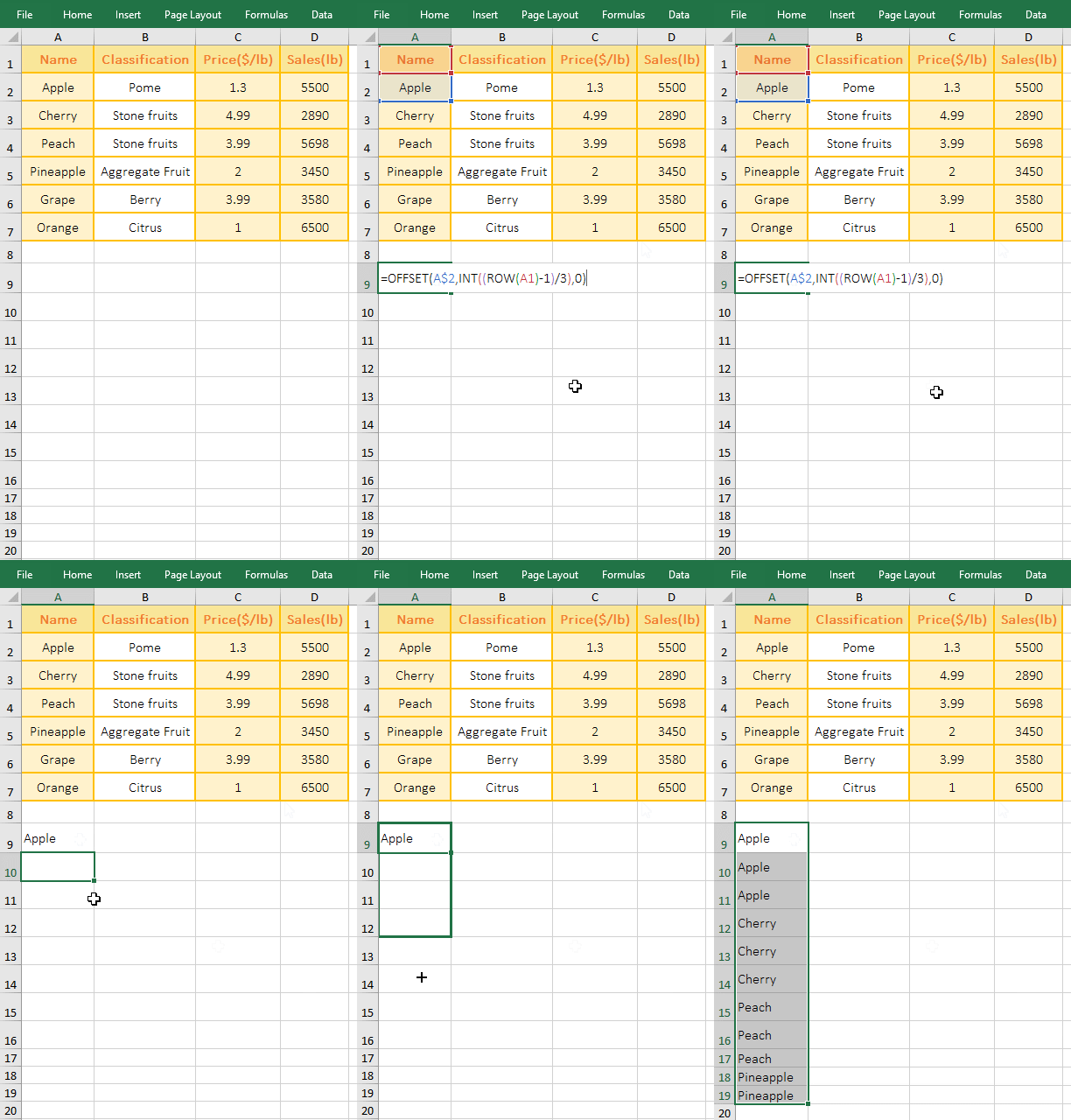
Figure 8

2. The formula =OFFSET(A$2,INT((ROW(A1)-1)/3),0) description:

A, ROW(A1) is used to return the Row_Num of A1. When dragging down, A1 will become A2, A3, etc., and then use the Row function to return their Row_Num.

B. 3 in the formula indicates the number of repetitions; INT((ROW(A1)-1)/3) is used to round the result of (ROW(A1)-1)/3, leaving only the integer part and not rounding off; for example: the result of (ROW(A1)-1)/3 is 0/3, then INT(0) returns 0; the result of (ROW(A4)-1)/3 is 4/3, then INT(4/3) returns 1.

C. The formula becomes =OFFSET(A$2,0,0), and finally uses OffSet function to return the reference to a cell 0 row under A2 and 0 column to right of A2, which is the "Apple" in A2. If A1 becomes A4, the formula becomes =OFFSET(A$2,1,0), and finally uses OffSet function to return the reference to a cell 1 row under A2 and column 0 to right of A2, which is "Cherry" in A3.

(IV) CountIf + OffSet + Match + CountIf function combination to achieve segmentation statistics

1. If you want to count the number of "employees" in any department. Double-click cell G2, copy the formula =COUNTIF(OFFSET(C1,MATCH(E2,B2:B9,),,COUNTIF(B2:B9,E2)),F2) to G2, press Enter, return to the statistical result 2; select cell E2, change "Technology Department" to "Finance", click G2, return to the  Employee of "Finance" statistical result 3; the operation process steps, as shown in Figure 9:

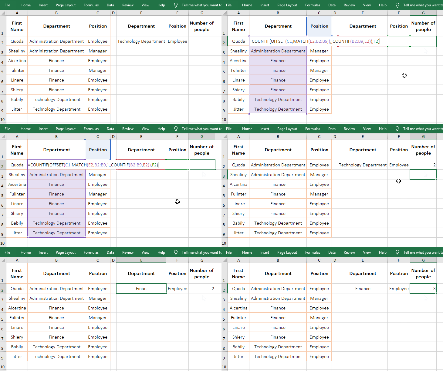
Figure 9

2. The formula =COUNTIF(OFFSET(C1,MATCH(E2,B2:B9,),,COUNTIF(B2:B9,E2)),F2) description:

A. MATCH(E2,B2:B9,) is used to return the position 3 of E2(ie "Technology Department") in B2 to B9. Match function also omits the last argument, and defaults to 0.

B. COUNTIF(B2:B9,E2) is used to count the number of E2(Technology Department) in B2 to B9, the result is 3, B2:B9 is the statistical range, and E2 is the criteria.

C. Then OFFSET(C1,MATCH(E2,B2:B9,),COUNTIF(B2:B9,E2)) becomes OFFSET(C1,3,,3), meaning that C1 is used as the reference, and it returns the reference to cells rows 3 under C1 and column 0 to right of C1 with height to 3, that is, returns C4:C6.

D. The formula becomes =COUNTIF(C4:C6,F2), and finally count the number of F2 (employees) in C4 to C6. There are only two employees in the administrative department, so the result 2 is correct.

Hint: The column that is counted must be sort.

(V) If + Or + CountIf + OffSet + Row function combination to achieve break code check

1. If you want to determine whether the garment is broken, assume that four consecutive sizes are not 0 as the same code, otherwise it is a code break. Double-click cell H2, copy  the formula =IF(OR(COUNTIF(OFFSET(A$1,ROW(A1),ROW($1:$3),,4),">0")>=4),"No","Yes") to H2, press Enter, return "Yes"; select H2, click on the cell fill handle to return whether the remaining clothing is broken; the operation steps, as shown in Figure 10:

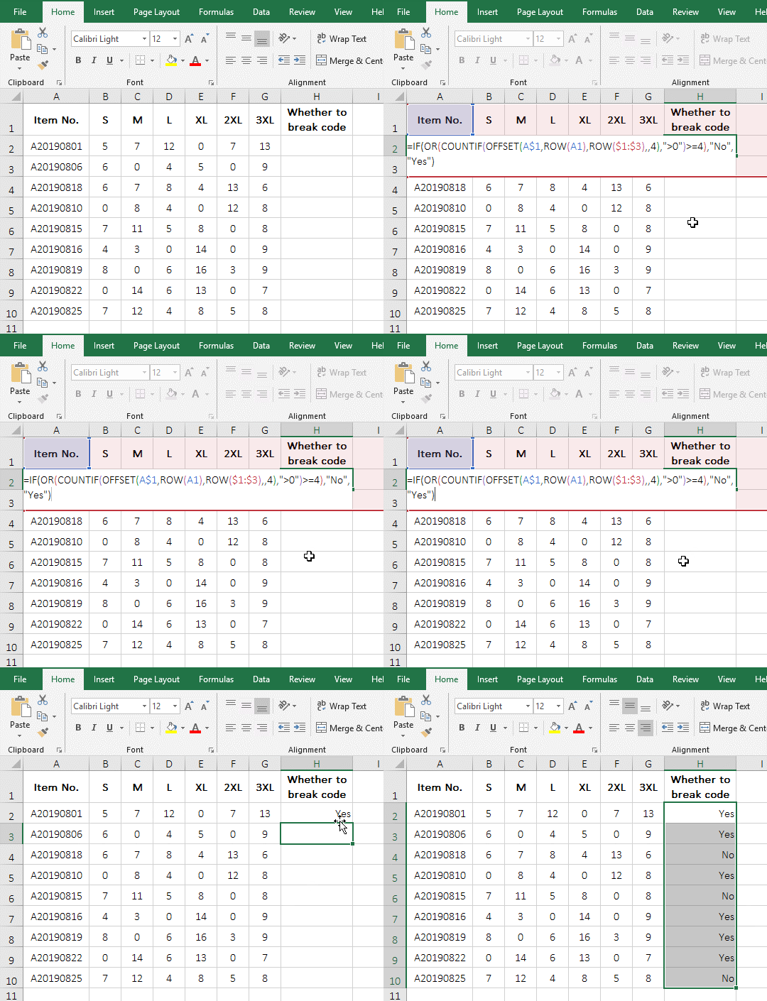
Figure 10

2. Formula =IF(OR(COUNTIF(OFFSET(A$1,ROW(A1),ROW($1:$3),,4),">0")>=4),"No","Yes") description:

A. A$1 has been explained in the above dynamic summation; ROW(A1) is used to return the Row_Num 1 of A1; ROW($1:$3) is used to return an array of 1 to 3, ie {1;2;3 };4 is the Width of the OffSet function, which is used to take 4 consecutive values in cells.

B. Why return an array of 1 to 3? After the above operation, OFFSET(A$1,ROW(A1),ROW($1:$3),,4) becomes OFFSET(A$1,1,{1;2;3},,4), since the argument Cols is an array, the first element 1 can only be fetched from the array for the first time, so OffSet function returns the reference to the cells 1 row under A1 and 1 column to right of A1 with width to 4 for the first time, That is, returns B2:E2; takes the second element 2 from the array for the second time, OffSet function the reference to cells  1 row under A1 and column 2 to right of A1 with width to 4 for the second time, ie C2:F2; similarly, OffSet function returns D2:G2 for the third time; takes an array of 1 to 3 to the last column of the table size(ie column G); OffSet function finally returns {#VALUE!;#VALUE!;#VALUE!}, and #VALUE! in the array represents B2:E2, C2:F2 and D2:G2.

C. Then COUNTIF(OFFSET(A$1,ROW(A1),ROW($1:$3),,4),">0") becomes COUNTIF({#VALUE!;#VALUE!;#VALUE!}," >0"), then, according to ">0", each reference range is counted. B2:E2 has a 0, so the statistical result is 3; C2:F2 and D2:G2 both have a 0, and the statistical results are also 3.

D. The formula becomes =IF(OR({3;3;3}>=4),"No","Yes"), then the first element 3 is taken from the array and compared with 4, since it is not established , so return False; continue to take the second and third elements, they are not true, also returns False; then the formula becomes =IF (OR{FALSE;FALSE;FALSE},"No","Yes"), due to the All elements in array are false, so if Or function returns FALSE, the formula becomes =IF(FALSE,"No","Yes"), and the condition of If is false, so it returns "Yes".