How to use Excel address function(7 examples, with Indirect,Sum,OffSet,Match and extract data)

The Address function returns the address of a cell specified by the row and column number in Excel, it can specify the type of reference, reference style, and worksheet to be referenced. There are four types of references, namely: absolute reference to column and row, absolute references to column and relative reference to row, relative reference to column and absolute reference to row, and relative reference to column and row.

Since the Address function returns the address of the cell in text mode, the result that is returned by it also needs to use the Indirect function to convert the text to a reference to the cell; then combine with OffSet, Match, Sum, Row, and Column to achieve the specific function. For example, Indirect + Address + Row + Column implements extracting data starting from the specified row, OffSet + Indirect + Address + Match can lookup data, Sum + OffSet + Indirect + Address can sum to multi-table.

I, The syntax of the Excel Address function

1. Expression: ADDRESS(Row_Num,Column_Num,[Abs_Num],[A1],[Sheet_Text])

2. Description:

A. Abs_Num is optional. If omitted or 1, it returns "absolute value"; if it is 2, it returns "absolute row number, relative column label"; if it is 3, it returns "relative row number, absolute column label"; if it is 4, it returns "relative value".

B. A1 is optional. If omitted or True, returns A1-style reference; if False, returns an R1C1-style reference, R is the row number, and C is the column number.

C. Sheet_Text is optional. If omitted, it means to reference the current worksheet; if you want to refer to the external worksheet, just write the worksheet name, such as Sheet2.

II, The examples of Excel Address function

(I) Omitting optional arguments

1. Double-click cell E2, copy the formula =ADDRESS(2,3) to E2, press Enter, return the reference result to the cell as $C$2; the operation procedure is as shown in Figure 1:

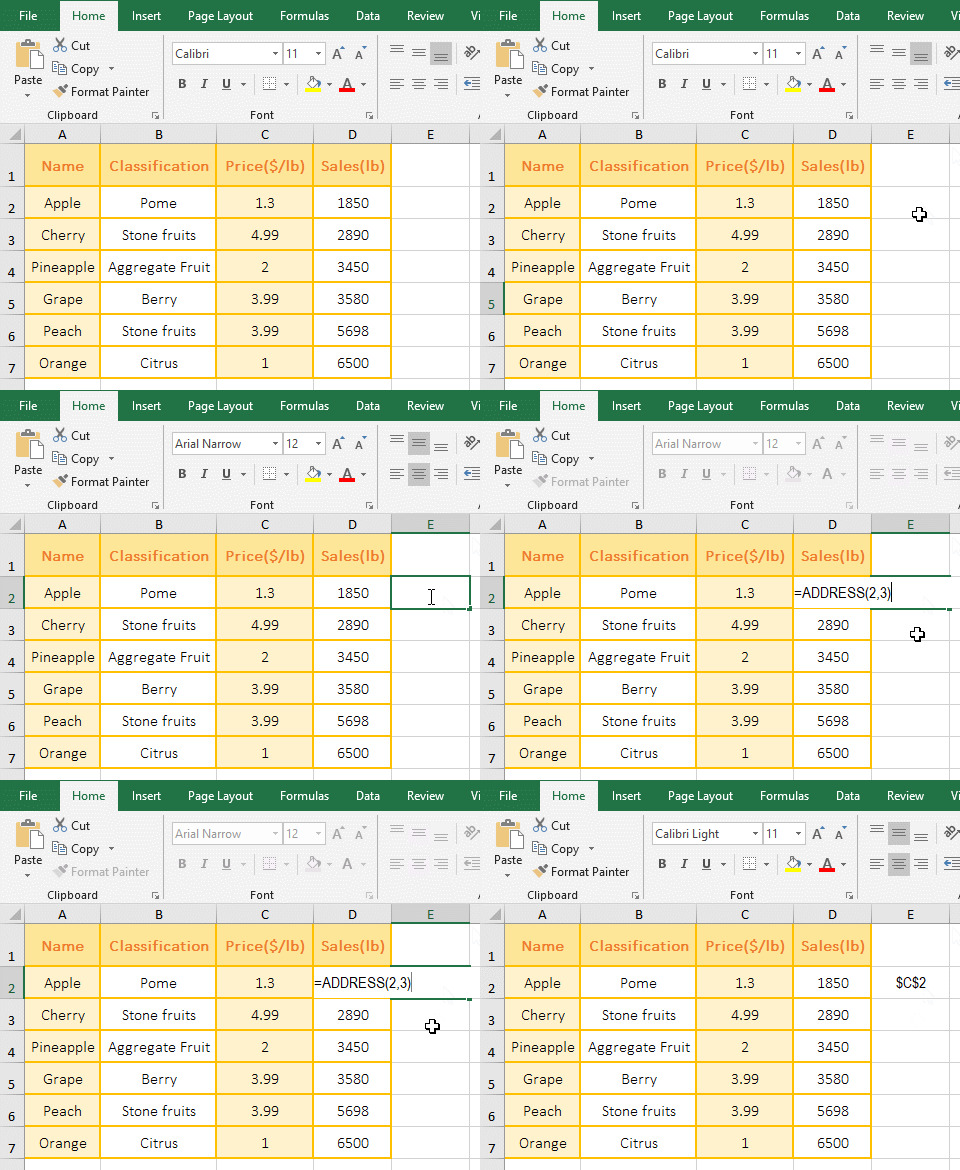
Figure 1

2. Formula description:

2 is the row number, indicating the 2nd row; 3 is the column number, indicating the 3rd column in formula=ADDRESS(2,3); the formula omits the last three arguments, Abs_Num(type of reference) is the third argument of the formula, if omitted, return the absolute value, that is, the absolute reference to the cell, such as returning the result $C$2; A1(reference style) is the fourth argument of the formula, if omitted, returns the A1-style reference; Sheet_Text(the name of the worksheet) is fifth argument of the formula, if omitted, returns to the current worksheet; the formula means: return an absolute reference to the cell at the intersection of the second row and the third column of the current worksheet in text, and return it with the A1-style reference.

(II) Return four types of reference

1. Double-click cell A11, copy the formula =ADDRESS(7,4,1) to A11, press Enter, return to $D$7; double-click B11, paste the same formula to B11, change 1 to 2 press Enter , return D$7; double-click C11, copy the same formula to C11, change 1 to 3, press Enter, return to $D7; double-click D11, copy the same formula to D11, change 1 to 4, press Enter, return to D7; the operation steps are as shown in Figure 2:

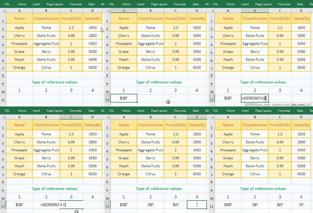
Figure 2

2. Formula description:

A. The formula =ADDRESS(7,4,1) means: return the reference to cell at the intersection of the 7th row and the 4th column with text, and return with "absolute reference", that is, return $D$7, $ means absolute reference, there are $ before column and row, indicating absolute reference to the column and row, that is, when dragging down or to the right, D7 will not become D8, D9, ..., will not become E7, F7,....

B. The third argument "type of reference" of formula =ADDRESS(7,4,2) is 2, which means "absolute row, relative column(ie absolute reference to row, relative reference to column)" and returning a reference to a cell with text, returns D$7. When dragging down, D7 does not change to D8, D9, ..., but when dragged to the right, D7 becomes E7, F7, ....

C. The third argument "type of reference" of formula =ADDRESS(7,4,3) is 3, which means "relative row, absolute column (ie, relative reference to row, absolute reference to column)" and returns a reference to the cell with text, which returns $D7. When dragged down, D7 will change to D8, D9, ..., but when dragged to the right, D7 will not become E7, F7, ....

D. The third argument "type of reference" of formula =ADDRESS(7,4,5) is 4, indicating that "relative"(that is, relative to the row and column)" and return a reference to the cell in text, that is, return D7, when dragging down, D7 will become D8, D9, ..., when dragging to the right, D7 will also become E7, F7, ....

(III) Examples of A1-style and R1C1-style reference

1. Double-click cell E2, copy the formula =ADDRESS(6,1,,1) to E2, press Enter, return $A$6; double-click E3, copy the same formula to E3, and change the following 1 to 0. press Enter, return to R6C1; the operation steps are as shown in Figure 3:

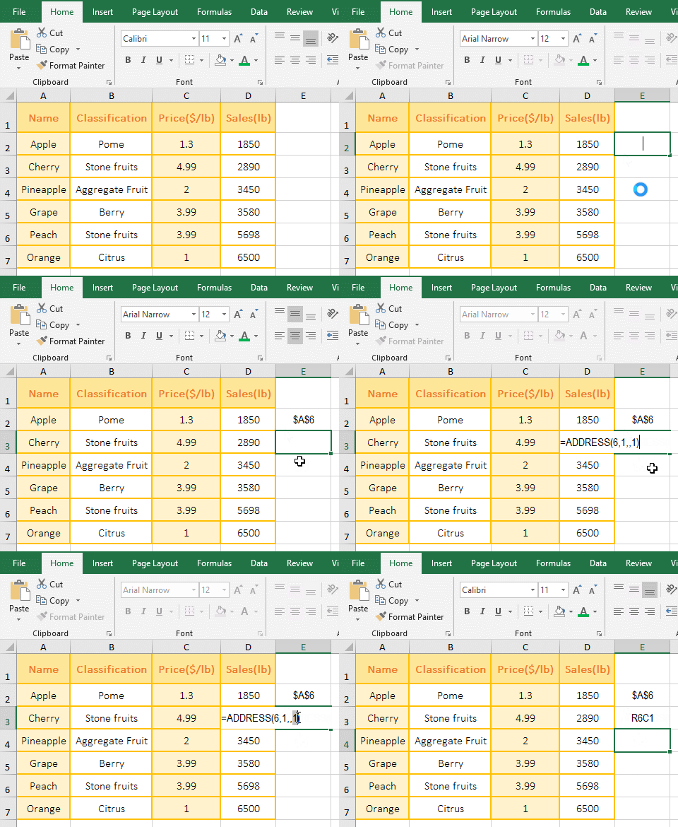
Figure 3

2. Formula description:

A. The formula =ADDRESS(6,1,1,1) is to return a reference to the cell at the intersection of 6th row and 1st column in text, the third argument is omitted, the default is returned by absolute reference, the fourth argument is 1(ie True), returned in A1-style, so return $A$6.

B. The formula =ADDRESS(6,1,,0) return also a reference to the cell at the intersection of 6th row and 1st column in the absolute reference and the text, the fourth argument is 0(ie False), represents returning in R1C1-style, so return R6C1.

(IV) Reference to the cell of an external worksheet

1. Reference another worksheet in the same document; the current sheet is "September", if you want to reference to D5 of another sheet "October"; double-click E2, and copy the formula =ADDRESS(5,4,,,"October") to E2, press Enter, return October!$D$5.

2. Reference one of the worksheets of the different documents; if you want to reference to D5 in the "Sales" in the "Clothes" document; double-click cell E3, and copy the formula =ADDRESS(5,4,,,"[clothes.xlsx]sales") to E3, press Enter, return to [clothes.xlsx]sales!$D$5; operation process steps, as shown in Figure 4:

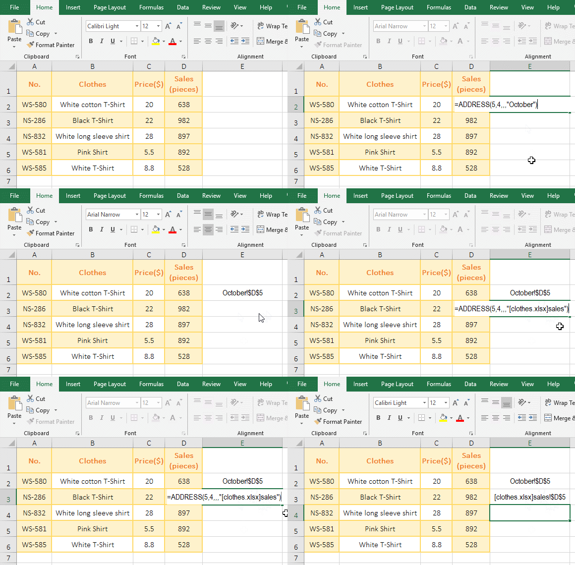
Figure 4

3. Formula description:

A. Formula =ADDRESS(5,4,,,"October") returns an absolute reference to D5 of another sheet "October" in the sheet "September" with text, since the two sheets are in the same document, Therefore, there is no need to add a document name in front of the sheet.

B. Formula =ADDRESS(5,4,,,"[clothes.xlsx]sales") is the absolute reference to D5 of the "Sales" in another document(ie "clothes.xlsx"). Since the document in which the formula is located is not the same document as the document in which contains the cell to be referenced, the "name of reference" must have the name of document and the name of worksheet and the name of document must have an extension, otherwise the document cannot be found, as in the formula "[clothes.xlsx]sales"; if you want to view the value in the cell to be referenced, you need to add the Indirect function, then the formula becomes =INDIRECT(ADDRESS(5,4,,,"[clothes.xlsx]sales")); In addition, the referenced document is opened and the formula returns the correct value, otherwise the reference error #REF! is returned.

III, The application examples of Excel Address function

(I) Indirect + Address + Row + Column combination extracts data starting from the specified row

1. If you want to extract data of arbitrary row from the third row. Double-click cell A9, copy the formula =INDIRECT(ADDRESS(ROW($A3),COLUMN())) to A9, press Enter, and return to "Cherry"; select A9 and move the mouse to the cell fill handle in the lower right corner of A9, after the mouse changes to bold black plus sign, hold down the left button, drag to the right, drag to D9, then extract the data of third row in the table; then drag down, how many rows, how many data of rows are extracted, such as drag four rows down, then extract the four data of rows in the table; the operation steps are as shown in Figure 5:

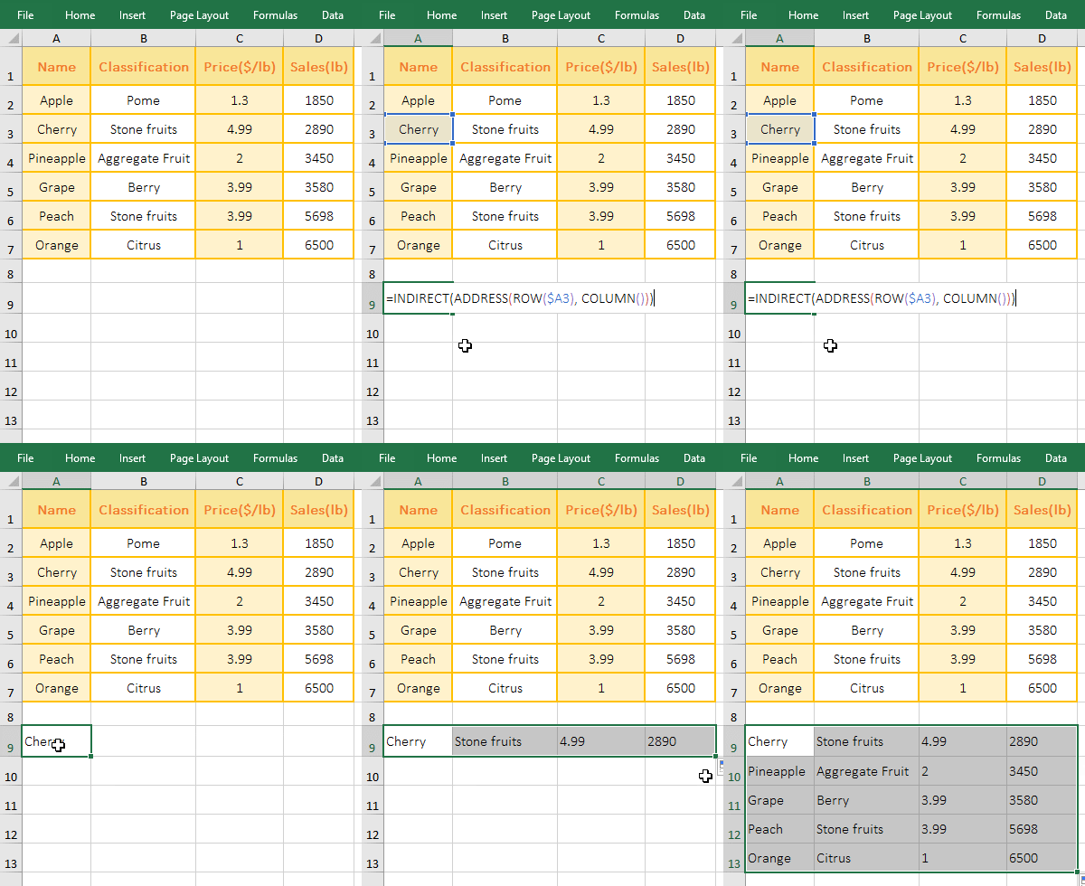
Figure 5

2. The formula =INDIRECT(ADDRESS(ROW($A3),COLUMN())) description:

A. $A3 means that the absolute reference to the column and relative to the row; when dragging down, A3 will change to A4, A5, etc. When dragging to the right, A3 will not change to B3, C3, etc.; The line number grows and the column number does not change.

B. ROW($A3) returns the row number 3 of A3, COLUMN() returns the column number 1 of the column in which contains the formula, then ADDRESS(ROW ($A3),COLUMN()) becomes ADDRESS(3,1), which returns the absolute reference to the cell at the intersection of third row and first column in text, which is "$A$3".

C. The formula becomes =INDIRECT("$A$3"), and finally returns a reference to the text "$A$3" by the Indirect function, which returns the content in A3.

D. When the formula is in B10, $A3 becomes $A4, ROW($A4) returns A4's row number 4; COLUMN() returns B10's column number 2; then the formula becomes =INDIRECT(ADDRESS(4,2)) , further calculation becomes =INDIRECT("$B$4"), and finally returns the content "Aggregate Fruit" of B4.

(II) OffSet + Indirect + Address + Match combination to lookup data(Excel address match)

1. If you want to find a Position by First Name. Double-click the cell B12, copy the formula =OFFSET(INDIRECT(ADDRESS(MATCH(A12,A1:A9,),1)),,2) to B12, press Enter, return to Jitter's position "Employee"; double-click A12, Change Jitter to Fulinter, and press Enter, then return to Fulinter's position as "Manager"; the process steps are as shown in Figure 6:

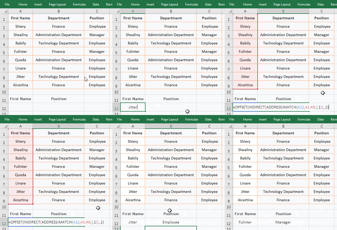
Figure 6

2. The formula =OFFSET(INDIRECT(ADDRESS(MATCH(A12,A1:A9,),1)),,2) description:

A. MATCH(A12,A1:A9,) is used to find A12 in A1:A9. It omits the last argument, the default is 0, which means exact match. The final result is 6.

B. Then ADDRESS(MATCH(A12,A1:A9,),1) becomes ADDRESS(6,1), since the latter three arguments are omitted, they all take the default value, so return the address of cell at the intersection of the sixth row and the first column with absolute reference, which returns "$A$6".

C. Since the Address function returns text, the Indirect function is also used to convert the text to a reference, ie INDIRECT("$A$6") returns $A$6.

D. The formula becomes =OFFSET($A$6,,2), and then, based on A6, returns the reference to the cell to the right of A6 with two columns, which returns a reference to C6, that is, the content "Employee" in C6 is returned. The OffSet function omits the second argument row number, the default value is 0; the fourth and fifth arguments height and width are also omitted, the height and width are the same as A6 by default.

(III) Sum + OffSet + Indirect + Address combination to sum multi-table

1. If you want to subtotal the sales of clothing from  September to November, the sales volume of each month is in a sheet, and the name of the sheet is named after the month. The current sheet is "September", select the "Sales subtotal" sheet, double-click cell B2, and copy the formula =SUM(OFFSET(INDIRECT(ADDRESS(1,4,,,A2)),1,,6)) to B2, press Enter, return to the summation result 3937; select B2, and then double-click the cell fill handle of B2 to return the sum of sales in October and November; the operation steps, as shown in Figure 7:

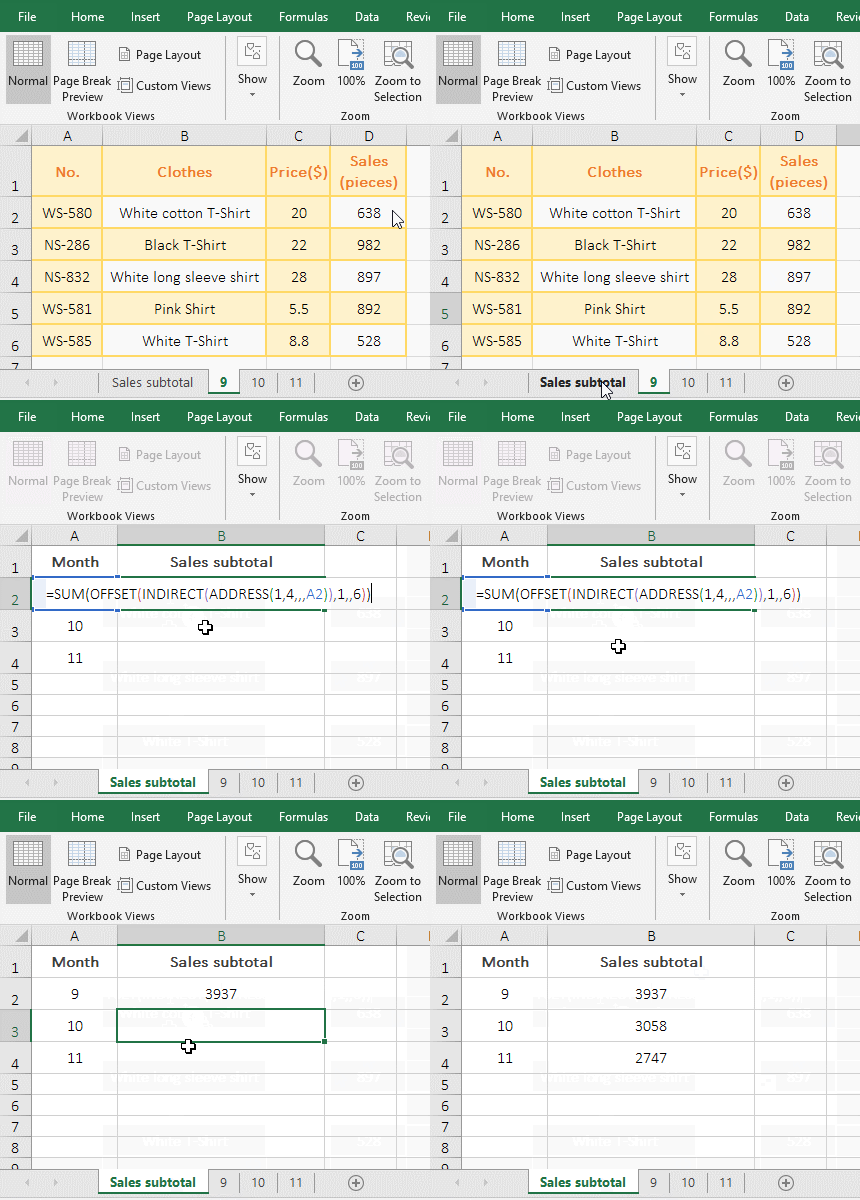
Figure 7

2. The formula =SUM(OFFSET(INDIRECT(ADDRESS(1,4,,,A2)),1,,6)) description:

A. The month in A2 is 10, then ADDRESS(1,4,,,A2) becomes ADDRESS(1,4,,,"10"), and then returns to the address of the cell at the intersection of the first row and the fourth column in the sheet "September" in absolute reference, that is, returns the text "'9'!$D$1".

B. Next, converts the text "'9'!$D$1" to a reference to the cell with the Indirect function, ie INDIRECT("'9'!$D$1"), which returns '9'!$D$1.

C. The formula becomes =SUM(OFFSET('9'!$D$1,1,,6)), further calculation, based on the D1 in the sheet "9", return the reference to cells row 1 under D1 and column 0 to right of D1 with height to 6 and width to 1, ie returns $D$2:$D$7.

D. The formula is further changed to =SUM('9'!$D$2:$D$7), and finally adds the values in D2:D7.