Generate Excel random number with Rand and RandBetween function(no duplicate and specified range)

You can generate random numbers by the Rand function or RandBetween function. The former are used to generate decimal random numbers from 0 to 1, and the latter are used to generate integer random numbers in a specified range. The Rand function can also generate a random number in a specified range, but use the formula =RAND()*(b-a)+a, and the generated random numbers are still a decimal.

You use the Rand or RandBetween function to generate random numbers, both may generate duplicate random numbers. If you need to generate non-repeated random numbers, you need to generate seeds first and then use the seeds to generate random numbers, or the random numbers are generated by Small + If + CountIf + Row + Int + Rand function. The random numbers that are generated by the Rand or RandBetween function are easy to change in the default case, if you need to generate constant random numbers, you need to convert them to numeric values.

I, Excel random number generation function syntax

(I) Rand function in excel

1. Expression: RAND()

2. Description:

A. Rand function is used to generate random numbers between 0 and 1. If you want to generate random numbers between a and b, you need to use RAND()*(b-a)+a; for example, to generate random numbers from 1 to 100, you can use the formula =RAND()*(100-1)+1.

B. The random number generated by the Rand function will change to another random number when the worksheet is calculated. If you want it to be not changed, enter the formula =RAND(), keep the edit state, and press F9 to turn the formula into a numerical value, see examples below.

(II) RandBetween function in excel

1. Expression: RANDBETWEEN(Bottom, Top)

2. Description:

A. RandBetween function is used to generate random numbers between any two specified numbers. The argument Bottom is the minimum value of the specified range, and Top is the maximum value of the specified range.

B. Like the Rand function, the random number generated by the RandBetween function will also become another random number when the worksheet is calculated. If the generated random number is required to remain unchanged, after entering the formula, press F9 to turn the formula into the valu.

II, How to use rand function in excel

(I) Generate a fixed Excel random number between 0 and 1, and how to stop random numbers from changing in excel

Select cell A1, enter formula =rand(), press Enter to return a random number of 0.872317939; double-click A1, press Enter, the random number becomes 0.11638895, when the formula is executed, the random number will change; double-click A1 again, press F9, then the formula turns to a random number 0.929025516988154, no matter how you double-click A1, the formula will not appear, and the random number will not change again; the operating process steps are shown in Figure 1:

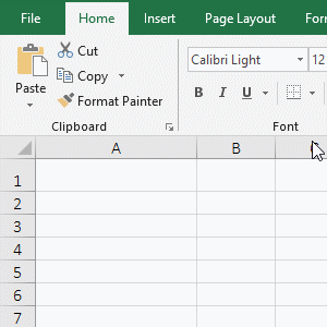
Figure 1

(II) Generate a Excel random number in a specified range

1. if you want to generate a random number between 100 and 1000. Double-click the cell A1, copy the formula =INT(RAND()*(1000-100)+100) to A1, and press Enter to return the random number 345. The operation steps are shown in Figure 2:

Figure 2

2. Formula =INT(RAND()*(1000-100)+100) explanation:

Generate random numbers between 100 and 1000 with the formula =RAND()*(b-a)+a, a is 100, b is 1000, but the random numbers generated by this formula are decimals. If you want to generate the random number for integer, the number is rounded with the Int function.

III, How to use RandBetween function in excel

(1) Generate a fixed integer random number in a specified range and the method of Excel randbetween stop changing

Suppose you want to generate a random number between 0 and 100. Double-click cell A1, copy the formula =RANDBETWEEN(0,100) to A1, and press Enter to return the random number 73; double-click A1, press Enter, the random number becomes 68, and when the formula is executed, the random number will also change; double-click A1 again, press F9 to change the formula to the value 4, and then double-click A1, the formula will no longer appear; the operation steps are shown in Figure 3:

Figure 3

(2) Generate random numbers between positive and negative numbers

Suppose you want to generate a random number between -100 and 100. Double-click cell A1, copy the formula =RANDBETWEEN(-100,100) to A1, and press Enter to return a random number -44; double-click A1 again, press Enter to return a random number 23; the operation steps are shown in Figure 4:

Figure 4

IV, The extended examples of Excel random number generation function

(I) How to fix random numbers in excel

There are two ways to generate a fixed random number in Excel. One is to enter the formula and press F9 to turn the formula into a value, which has been described above. The other method is to copy the generated random numbers into the values, the generated random numbers can be converted into fixed values in batches. The specific method is as follows:

Double-click cell A1, there is a formula for generating random numbers, press Enter to generate new random numbers; select A1:B9, press Ctrl + C to copy; the current tab is "Home", click "Paste" in the top left of the screem, select the "Value" icon under "Paste Values"and in the pop-up options, the formula for generating random numbers in all selected cells will be converted to numeric values, and double-click A1 again, there is no formula; the operation steps are shown in Figure 5:

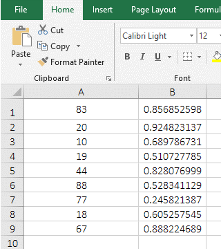
Figure 5

(II) Excel generate unique random numbers(ie Excel random number generator no duplicates)

(1) Generate seeds first, and then generate unique random numbers with the seeds

1. Generate non-repeating decimal random numbers

A. Generate seeds. Double-click cell A1, copy the formula =RAND() to A1, and press Enter to generate a decimal random number; select A1, move the mouse to the cell fill handle at the bottom right of A1, hold down the left button, and drag down to A9, the cells passed through are filled by the random numbers. the generated random numbers is the same, press Ctlr + S to save, then they will be updated to a different random numbers.

B. Generate a unique random number. Double-click B1, copy the formula =RAND() to B1, enter * A1, press Enter to return a new random number; select B1, move the mouse to the cell fill handle of B1, and double-click the left button after the mouse becomes the bold black plus sign, then B2:B9 are filled by the  no duplicate random numbers; the operation steps are shown in Figure 6:

Figure 6

2. Generate unique random integers in a specified range

A. If you want to generate a random number between 50 and 100. Double-click cell A2, copy the formula =RANDBETWEEN(50,100) to A2, press Enter to generate a seed random number, and drag down to generate other seed random numbers;

B. Double-click B2, copy the formula =INT(RANDBETWEEN(50,100)*A2/100) to B2, and press Enter to generate a random number. Double-click the cell fill handle of B2 to generate other random numbers. The operation steps, see screenshot in Figure 7:

Figure 7

C. Formula =INT(RANDBETWEEN(50,100)*A2/100) explanation:

First, generate a random number of 50 to 100 with RANDBETWEEN(50,100), then use this random number to multiply the seed random number in A2, and then divide by 100(because the multiplication of the two 50 to 100 values has increased by 100 times, so to reduce it by a factor of 100), finally round with the Int function.

Hint: generating seeds first and then using seeds to generate random numbers cannot guarantee that the generated random numbers will not be repeated. If a unique random number is required to be generated, the following method is required.

(2) Generate non-repeating random numbers with the Small + If + CountIf + Row + Int + Rand function

A. If you want to generate unique random numbers between 1 and 12. Double-click cell A2 and copy the formula =SMALL(IF(COUNTIF(A$1:A1,ROW($1:$12))=0,ROW($1:$12)),INT(RAND()*(12-ROW(1:1))+1)) to A2, press Ctrl + Shift + Enter to generate a random number 3; move the mouse to the cell fill handle of A2, after the mouse becomes a bold black plus sign, drag down to A13, then the values ia A2:A13 will become the random numbers from 1 to 12; the operation process steps are shown in Figure 8:

Figure 8

B. Formula =SMALL(IF(COUNTIF(A$1:A1,ROW($1:$12))=0,ROW($1:$12)),INT(RAND()*(12-ROW(1:1))+1)) explanation:

a. A$1 means relative reference to column, absolute reference to row($ means absolute reference), when dragged down, A1 will not become A2, A3, etc.; when dragged to the right, A1 will become B1, C1, etc. A1 indicates that the columns and rows are relative references, when dragged down, A1 will become A2, A3, etc.; when dragged to the right, A1 will become B1, C1, etc.

b. A$1:A1 is used to return all the values from the current cell to the dragged cell; when the formula is in A2, A$1:A1 returns A1, and A1 is empty, so it returns 0; when the formula is in A3, A$1:A1 becomes A$1:A2, which returns the values in A1 and A2 as an array, that is, returns {0;2}; and so on.

c. $1 means an absolute reference to the row. When dragging down, 1 will not become 2, 3, etc.; $12 and $1 have the same meaning; ROW($1:$12) is used to return an array of 1 to 12, that returns {1;2;3;4;5;6;7;8;9;10;11;12}.

d. When the formula is in A2

COUNTIF(A$1:A1,ROW($1:$12)) becomes COUNTIF(A1,{1;2;3;4;5;6;7;8;9;10;11;12}), A1 is the counted range of the number, the array is a criteria. When executed, each element in the criteria array is counted in A1. The first execution, the first element(1) of the criteria array is taken, since the value of A1 is 0, therefore, the counted result is 0; the second execution, 2 is taken, and the counted result is 0; the rest and so on; and finally returns {0;0;0;0;0;0;0;0;0;0;0;0};

Then COUNTIF(A$1:A1,ROW($1:$12))=0 becomes {0;0;0;0;0;0;0;0;0;0;0;0}=0, then, take each element in the array is compared with 0, if it is equal, it returns True, otherwise it returns False, and finally returns {TRUE;TRUE;TRUE;TRUE;TRUE;TRUE;TRUE;TRUE;TRUE;TRUE;TRUE;TRUE};

Then IF(COUNTIF(A$1:A1,ROW($1:$12))=0,ROW($1:$12)) becomes IF({TRUE;TRUE;TRUE;TRUE;TRUE;TRUE;TRUE;TRUE;TRUE;TRUE;TRUE;TRUE},
{1;2;3;4;5;6;7;8;9;10;11;12}), when executed, each element in the criteria array of IF is taken out in sequence, if it is True, returns the element of the second array corresponding to it, otherwise returns False; since all elements of the criteria arrays are True, returns {1;2;3;4;5;6;7;8;9;10;11;12};

1:1 indicates a relative reference to the row. When you drag down, 1:1 will become 2:2, 3:3, etc.; ROW(1:1) returns the row number 1 of the first row; 12-ROW(1:1) returns 11, 12 is the maximum for generating random numbers in the specified range;

RAND() is used to return a decimal random number from 0 to 1. If it returns 0.146737187519064, then INT(RAND()*(12-ROW(1:1))+1) becomes INT(0.146737187519064 * 11 + 1), further calculation, it becomes INT(1.61410906270971 + 1), then rounded with the Int function, the result is 2;

Then the formula becomes =SMALL({1;2;3;4;5;6;7;8;9;10;11;12},2), and returns the 1st smallest number in the array with the Small function, that returns 2.

e. When the formula is in A3

COUNTIF(A$1:A2,ROW($1:$12)) becomes COUNTIF(A$1:A2,{1;2;3;4;5;6;7;8;9;10;11;12})); when executed, each element in the criteria array is counted in A1:A2, since A1 is 0 and A2 is 2, A1:A2 returns {0;2}; the first execution, 1 is taken from the criteria array, because there is no 1 in the array {0;2}, so it returns 0; the second execution, 2 is taken from the criteria array, because there is 2 in the array {0;2}, it returns 1; and so on, and finally returns {0;1;0;0;0;0;0;0;0;0;0;0};

Then COUNTIF(A$1:A2,ROW($1:$12))=0 becomes {0;1;0;0;0;0;0;0;0;0;0;0}=0, and the calculation result is {TRUE;FALSE;TRUE;TRUE;TRUE;TRUE;TRUE;TRUE;TRUE;TRUE;TRUE;TRUE};

Then IF(COUNTIF(A$1:A2,ROW($1:$12))=0,ROW($1:$12)) becomes IF({TRUE;FALSE;TRUE;TRUE;TRUE;TRUE;TRUE;TRUE;TRUE;TRUE;TRUE;TRUE},{1;2;3;4;5;6;7;8;9;10;11;12}), further calculation returns {1;FALSE;3;4;5;6;7;8;9;10;11;12}; the remaining steps are the same as for the formula in A2.

C. If you want to generate random numbers in other ranges(such as random numbers from 5 to 10), you only need to change the formula above. The formula can be written as follows:

=SMALL(IF(COUNTIF(B$5:B5,ROW($5:$10))=0,ROW($5:$10)),INT(RAND()*(10-ROW(5:5))+1))

Copy the formula to B6, press Ctrl + Shift + Enter to generate a random number, and then drag it down to B11, then generate 5 to 10 unique random numbers; the operation process steps are shown in Figure 9:

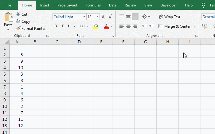
Figure 9