Excel Countifs formula examples, with And, Or, ? and * in Criteria

The CountIfs function is used to count the number of times two or more criteria are met at the same time in excel, and the CountIf function is used to count the number of times one criteria is met. The CountIfs function argument consists of a criteria range/criteria pair, at least one criteria range/criteria pair, at most 127 criteria range/criteria pairs.

In most cases, the CountIfs function itself can complete statistics that satisfy multiple Criteria, but it cannot complete the statistics of the "Or relationship"(Or Criteria); if you want to implement this function, you need to combine it with the Sum function. In addition, if you want to count the number of ranges that are not fixed, you need to use CountIfs + OffSet.

I, Excel CountIfs function syntax

1. Expression: COUNTIFS(Criteria_Range1, Criteria1, [Criteria_Range2, Criteria2], ...)

2. Description:

A. A Criteria range and a Criteria form a Criteria range/Criteria pair of CountIfs function. There must be at least one Criteria range/Criteria pair, There can be at most 127 Criteria range/Criteria pairs; each Criteria is "AND" relationship, if there are two Criteria, requires that both Criteria be met at the same time.

B. Criteria can be numbers, text(eg "employee"), a reference to a cell or references to cells, expressions(eg: ">=100"), and there can be functions in the Criteria(eg: "<="&Average(A2:A8))).

C. You can use the wildcard question mark(?) and asterisk(*) in the Criterai. The question mark indicates any character. The asterisk indicates one or a string of characters. If you want to find the question mark or asterisk, you need to add an escape character ~ before them.  For example: find ?, the expression should be written like this ~?; look for *, the expression should be written like this ~*.

D. If multiple Criteria ranges are referenced at the same time, the number of rows and columns of each Criteria range must be the same, but they do not have to be adjacent, otherwise the return value is errro #VALUE!.

C. If the Criteria is a reference to an empty cell, the CountIfs function will return 0.

II, The examples of Excel CountIfs function

(I) The Criteria is text and there is only one the Criteria range/Criteria pair

1. If you want to count the number of employees whose "Performance" is rated as "More excellent" in the table. Double-click the cell D9, copy the formula =COUNTIFS(D2:D9,"More excellent") to D9, press Enter, return to the counted result 3; the process steps, as shown in Figure 1:

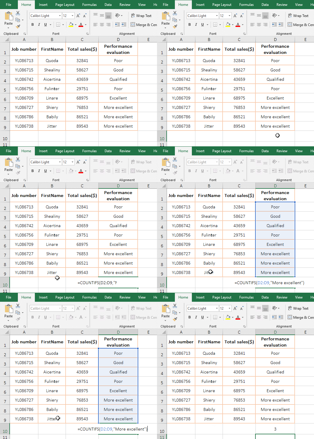
Figure 1

2. Formula description:

D2:D9 is the Criteria range, and "More excellent" is the Criteria in the formula =COUNTIFS(D2:D9,"More excellent"), meaning: the number of "Performance is rated as More excellent" is counted in D2 to D9; in general, One Criteria often uses the CountIf function, and two or more Criteria use the CountIfs function.

(II) Countifs examples with 2 conditions: the Criteria is an expression or with a function and there are two Criteria range/Criteria pairs

1. If you want to count the number of fruit whose price is more than 3 $/lb and the sales is greater than or equal to the average. Double-click the cell D8, copy the formula =COUNTIFS(C2:C7,">3", D2:D7,">="&AVERAGE(D2:D7)) to D8, press Enter, return to the counted result 1; as shown in Figure 2:

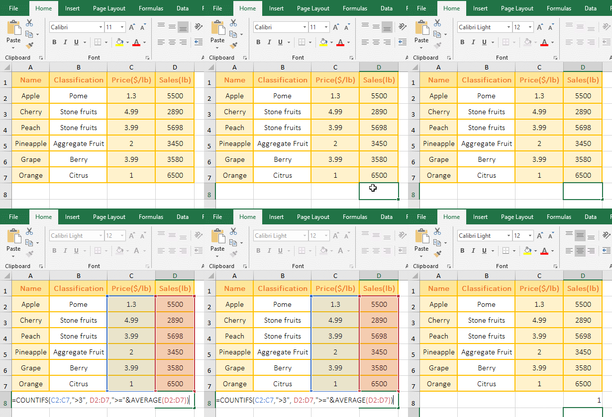
Figure 2

2. Formula =COUNTIFS(C2:C7,">3", D2:D7,">="&AVERAGE(D2:D7)) explanation:

The first Criteria range/Criteria pair is C2:C7,">3", used to find all values above 3 in C2:C7; the second Criteria range/Criteria pair is D2:D7,">="&AVERAGE(D2:D7), used to find the values which the "Sales" is greater than or equal to the average in D2:D7, AVERAGE(D2:D7) is used to calculate the average of "Sales", the concatenate operator & is used to connect ">=" with the average. Finally, the values that satisfy both the first and the second Criteria are selected as counted results.

(III) The Criteria is a reference to an empty cell, and the CountIfs function will return 0.

Double-click the cell C9, copy the formula =COUNTIFS(C2:C8,A8) to C9, press Enter to return to the counted result 0; select C9, hold down Alt, press M and V respectively to open the "Evaluate Formula" window, press Enter. A8 returns 0, indicating that when the Criteria is an empty cell, the CountIfs function treats its value as 0; the operation steps are as shown in Figure 3:

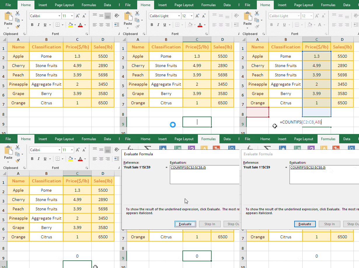
Figure 3

(IV) Criteria are empty and not empty

1. If you want to count the number of values which the size S is not empty and L is empty in the clothing size table. Double-click the cell B11, copy the formula =COUNTIFS(B2:B10,"<>",D2:D10,"") to B11, press Enter, return to the counted result 2; the operation steps, as shown in Figure 4:

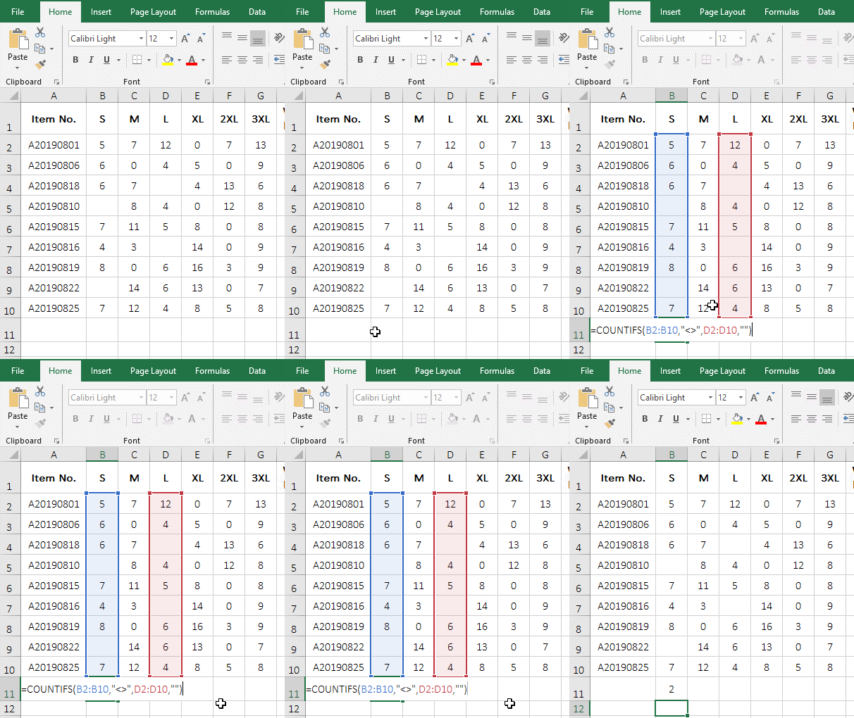
Figure 4

2. formula =COUNTIFS(B2:B10,"<>",D2:D10,"") description:

The first Criteria "<>" means not empty, it can also be expressed as "<>"&""; the second Criteria "" means empty in the formula.

(V) With wildcards ? and * in the Criteria

1. If you want to count the number of clothes whose name start with "Pink" and end with "Shirt" and only consist of ten characters. Double-click the cell B9, Copy the formula =COUNTIFS(B2:B8,"Pink*",B2:B8,"*Shirt",B2:B8,"??????????") to B9, press Enter, return to the counted  result 1; the operation steps, as shown in Figure 5:

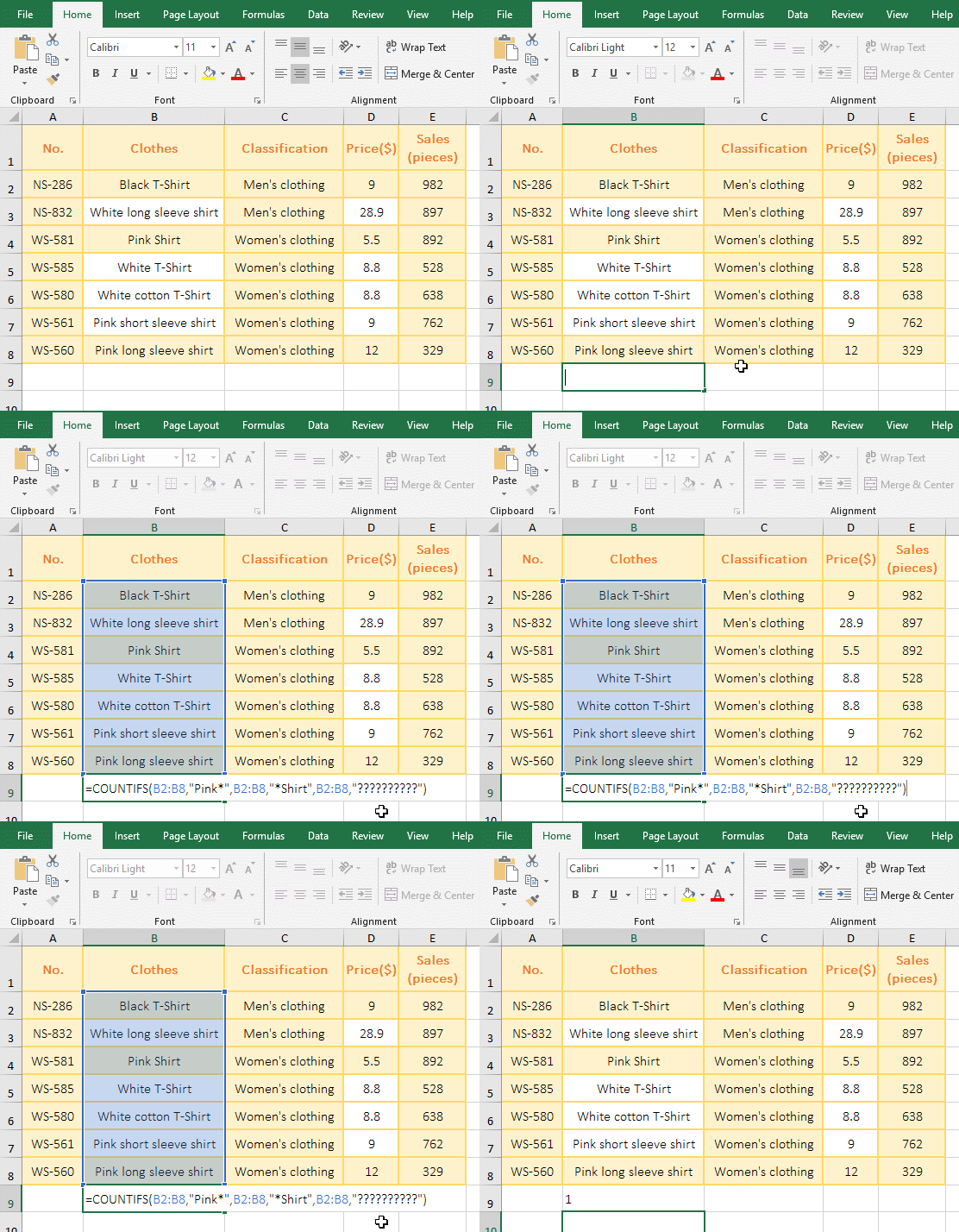
Figure 5

2. Formula =COUNTIFS(B2:B8,"Pink*",B2:B8,"*Shirt",B2:B8,"??????????") explanation:

The three ranges in the formula are B2:B8; the Criteria "Pink*" means to start with "Pink", * means any one or more characters; the Criteria "*Shirt" means to start with any one or more characters but to end with "Shirt"; the Criteria "??????????" means consisting of only ten characters.

III, Excel Countifs formula examples

(I) CountIf + OffSet function combination returns the reason for the error

1. Double-click the cell A10 and copy the formula =COUNTIFS(OFFSET($A$1,1,1,6,1),">600",OFFSET($A$1,2,2,7,1),">600") to A10, press Enter, return value error #VALUE!; select A10, hold down Alt, press M and V once, open the "Evaluate Formula" window, press Enter "Evaluate" until the formula changes for COUNTIFS($B$2:$B$7,">600", $C$3:$C$9,">600"); close the "Evaluate Formula" window, double-click B10, and change the formula to =COUNTIFS(OFFSET($A$1,1,1,8,1),">600", OFFSET($A$1,1,2,8,1),">600"), press Enter, return counted result 3, the same method open the "Evaluate Formula" window and press Enter to evaluate until the formula changes to COUNTIFS($B$2:$B$9,">600", $C$2:$C$9,">600"); As shown in Figure 6:

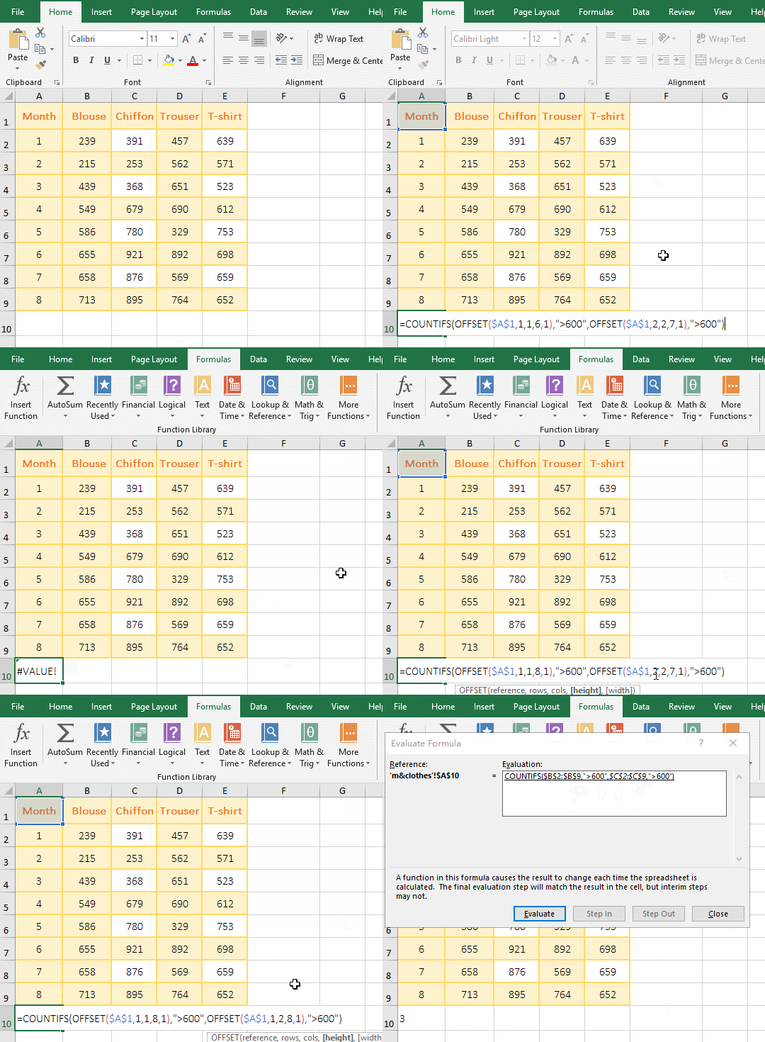
Figure 6

2. Formula description:

A. In the formula, OFFSET($A$1,1,1,6,1) is used to return a reference to a cell with 1 row under A1 and 1 column to right of A1 and height to 6 and width to 1, that is, return a reference to B2:B7; $A$1 means an absolute reference to A1, and A1 will never change whether dragging it to the right or dragging it to the right.

B. OFFSET($A$1, 2, 2, 7, 1) is used to return a reference to a cell with 2 rows under A1 and 2 columns to right of A1 and height to 7 and width to 1, that is, return a reference to C3:C9.

C. The formula becomes =COUNTIFS($B$2:$B$7,">600", $C$3:$C$9,">600"), the number of rows in Criteria range $B$2:$B$7 and $C$3:$C$9 is different, and the CountIfs function requires the number of rows and columns in the Criteria range to be the same, so the formula returns the error value #VALUE!.

D. After changing the formula to =COUNTIFS(OFFSET($A$1,1,1,8,1),">600", OFFSET($A$1,1,2,8,1),">600"), the two OffSets return the same number of rows and columns (that is, both are $B$2:$B$9), so they can return the correct statistics.

(II) Sum + CountIfs function combination to achieve statistics that satisfy both And and Or Criteria

1. If you want to count the total number of employees in the Administration and Finance Departments. Double-click the cell B10 and copy the formula =SUM(COUNTIFS(C2:C9,"employee",B2:B9,{"Administration Department","Finance"})) to B10, press Enter, return to 4, Operation process steps, as shown in Figure 7:

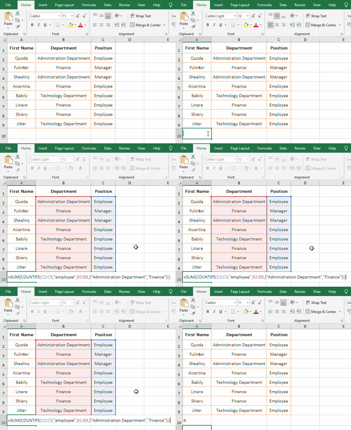
Figure 7

2. The formula =SUM(COUNTIFS(C2:C9,"employee",B2:B9,{"Administration Department","Finance"})) description:

A. The second Criteria of the formula is the array {"Administration Department", "Finance"}, which means to count the employees of "Administration Department and Finance" in B2:B9; when executing, first count the number of employees(the result is 1) in the "Administration Department", and then count the number of employees in the "Finance"(result is 3), finally CountIfs returns the array {3,1}.

B. The formula becomes =SUM({1,3}), and finally adds each elements in the array, the result is 3; if Sum is not used, only the one that satisfies the first Criteria in the array {"Administration Department", "Finance Department"} is returned.