How to make an excel spreadsheet, with the top 10 knowledge(Basic tutorial for create a table)

How to make an excel spreadsheet? Excel spreadsheets contain a lot of knowledge. Usually, you need to know the top 10 knowledge when you create a spreadsheet: create a new table, adjust the row height and column width, insert rows, columns and cells, delete rows, columns and cells, move rows, columns and cells, and edit the text in table, format cells, add borders for table and cells, sum and average, they are basic tutorial for create a table in excel and shared by specific examples in this article.

In the top 10 knowledge of the basic operation of the above Excel table, create a new table, adjust the row height and column width, insert, delete, move the row and column and cell have a variety of methods, and have shortcut keys; other five aspects of knowledge also have several methods, some of which are less; some only introduce one or two of the various methods, and more detailed methods are put into the special articles, such as sum and average.

I, How to make an excel spreadsheet

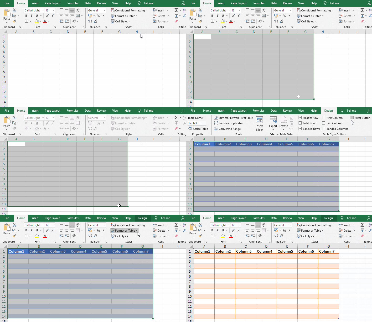
1. Move the mouse to the cell A1, hold down the left button and drag to the lower right corner, select the number of rows and columns to be created in the new table, for example, select 13 rows and 7 columns; press the shortcut key Ctrl + T to open the "Create Table" dialog, the selected range is automatically filled into the input box under "Where is the data for your table", press Enter(or click "OK") to create a 14-row, 7-column table, and default to blue table style, switch to the "Design" tab at the same time; click the "Filter button" to remove the check mark in front of it, then the filter box in the header row of each column in the table is removed; select the "Home" tab, click "Format as Table ", select a style in the pop-up table style, such as "Light Orange,table style color 17", the selected style is applied to the table; the operation process steps, see screenshot in Figure 1:

Figure 1

2. Select the "Insert" tab and click "Table" to open the "Create Table" dialog.

3. A1 represents the cell at the intersection of the first column and row, A represents the first column, and 1 represents the first row. In addition, select 3 rows and 7 columns can be represented by A1:G3, which is represented by a cell in the upper left corner and the lower right corner of the range to be selected.

4. If you want to modify the table style, you can click "Format as Table" again, and select another style in the pop-up style; if the style is not satisfied, you can fill the background color and border of the table yourself, it will be introduced below.

Tip: New table is created with the "Create Table" or after the table is applied in a table style, you can't sort and filter. In this case, you can convert the table into a range, see screenshot in Figure 2:

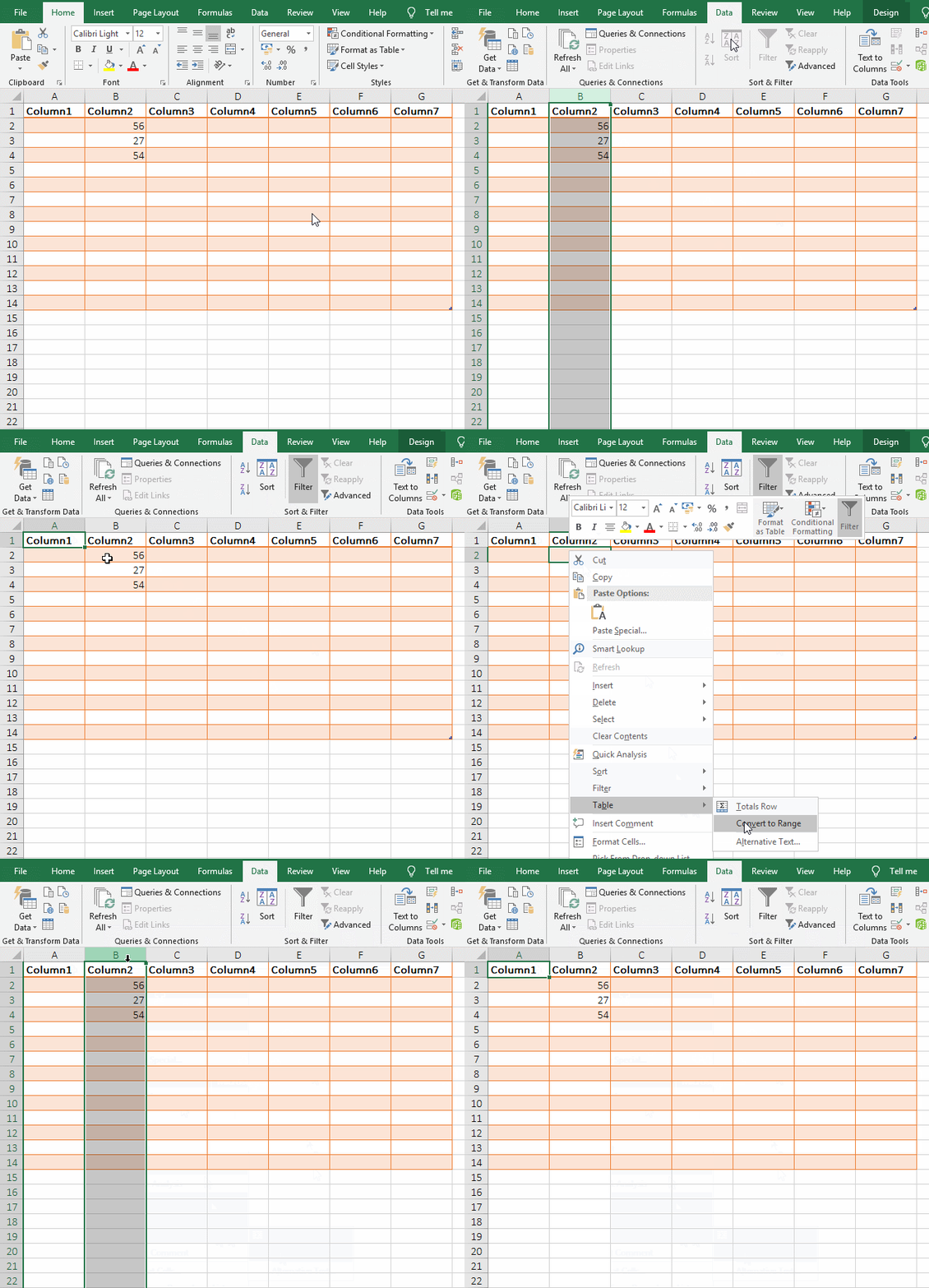
Figure 2

Demonstration process step description: Click the letter B to select column B, select the "Data" tab, "Sort and Filter" are grayed out and not selectable; right-click the table, select "Table" → "Convert to Range" in the pop-up menu, click "Yes" in the pop-up dialog, the table will be converted to range, and column B will be selected again, "Sort and Filter" are available.

II, How to adjust the row height or column width in excel

(I) How to adjust row height in excel

Method 1: Adjustment with right-click

Click the first row number 1 to select it, hold down the left button of mouse and drag down until the last row to select the entire table, right-click on one of the row numbers, select "Row Height" in the pop-up menu, open "Row Height" dialog, enter 22, press Enter, then all the row height of the table becomes 22, the operation steps, as shown in Figure 3:

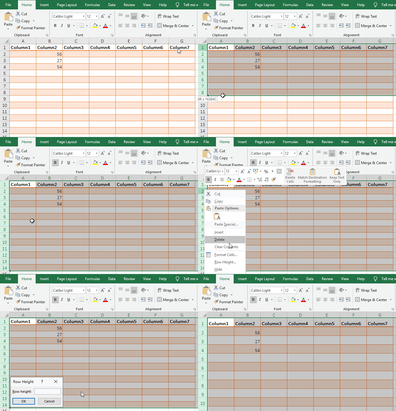
Figure 3

Tip: After clicking the first row to select it, hold down Shift and click the last row to select the entire table. If you don't want to select the entire table, for example, only the first three rows are selected, just click the third row.

Method 2: Adjustment with shortcut keys

Select the first row, hold down Shift, click the third row number 3, select the first three rows; press Alt, press H once, press O once, press H once, open the "Row Height" dialog, enter 28, Click "OK" or press Enter, the row height of the first three rows will become 28; the operation steps are as shown in Figure 4:

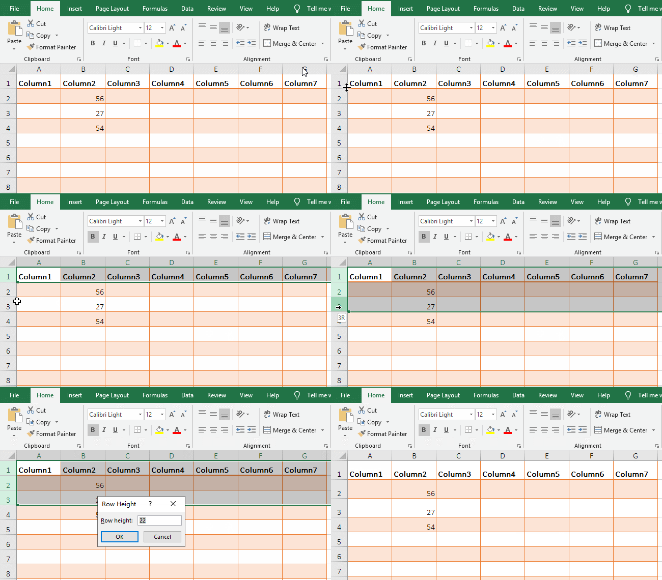
Figure 4

Method 3: Adjustment by dragging down

If you want to adjust the row height of row 4. Move the mouse to the lower line of the 4th row number, the mouse becomes a cross with double arrows in the vertical direction, hold down the left button, drag down, the row goes high; the same way adjust the row height of the 5th and 6th row; when dragging down, the row goes high; when dragging up, the row height becomes smaller; the operation steps are as shown in Figure 5:

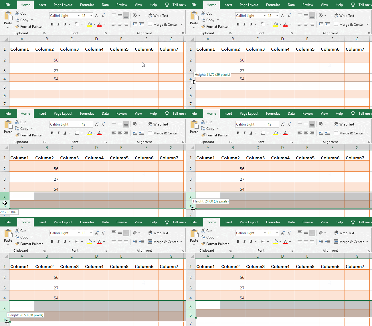
Figure 5

(II) How to adjust column width in excel

1. There are also three ways to adjust the column width, they are the same as adjusting the row height. The following is a list of methods for right-click and drag-and-drop adjustment. The operation steps are as shown in Figure 6:

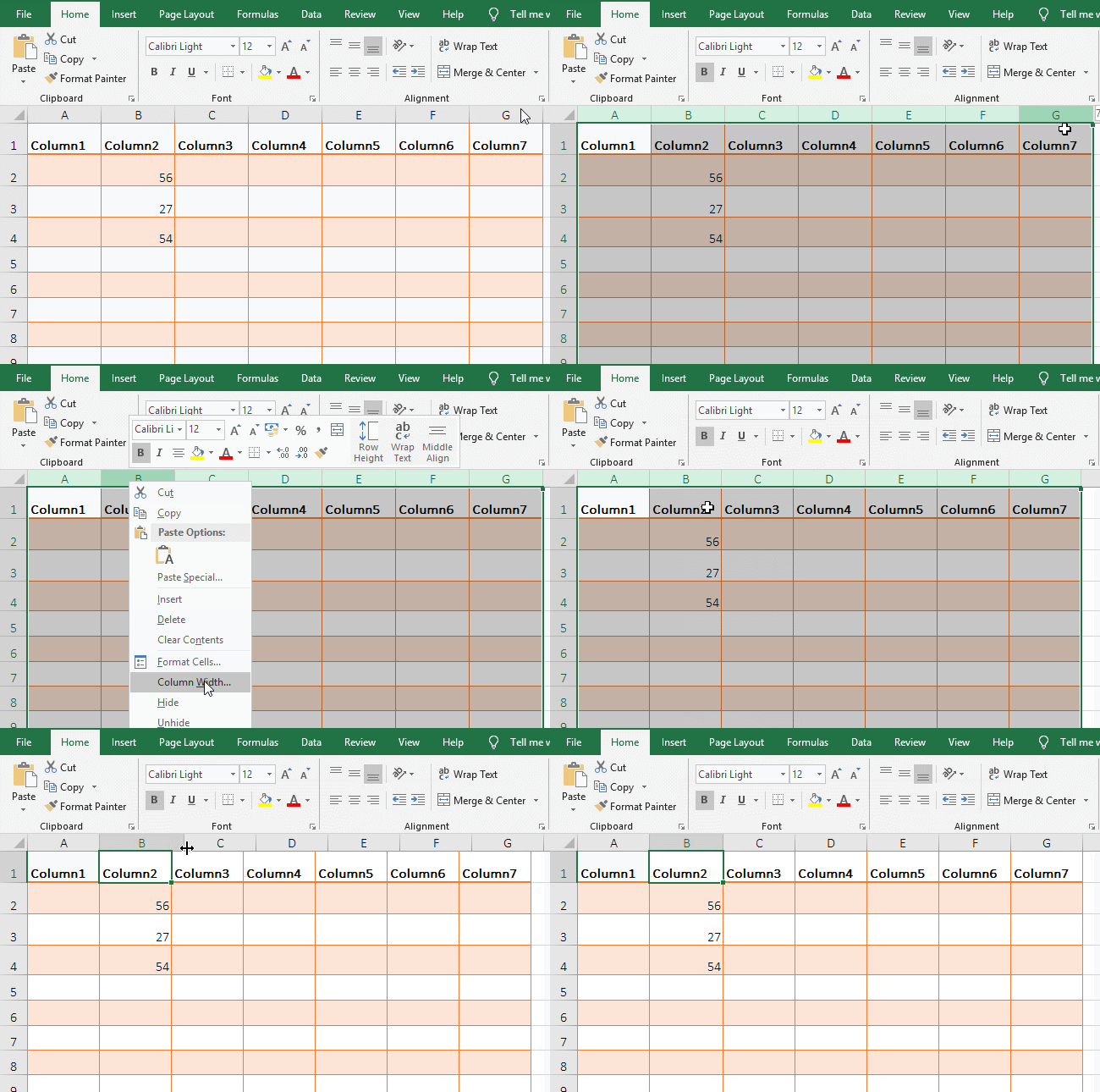
Figure 6

2. The operation process step description: Click A to select the first column, hold down Shift, click the G of the last column, select all the columns of the table; right click on one of the column numbers, select "Column Width" in the pop-up menu, pops up the "Column Width" dialog, enter 10, press Enter, then all the column widths of the table will become 10; move the mouse to the right line of the second column B, the mouse will become the cross with the horizontal arrow, press hold the left button, drag to the right, widening the column width; drag to the left, and narrow the column width.

Tip: Open the "Column Width" setting dialog can also press the shortcut key Alt + H + O + W. The key press method is: press and hold Alt, press H, O, W in order.

III, How to insert rows and columns, including inserting multiple rows and columns and multiple cells at a time

(I) How to insert rows?

1. How to insert a row in excel? Right click on the 4th row number, select "Insert" in the pop-up menu, insert a row in the 4th line, the original 4th row is moved down; click the "Brush" icon in the lower left corner of the newly inserted row, select "Format Same As Below" in the option, the new row will automatically set the same as format(such as pink) the row below; the operation steps, see screentshot in Figure 7:

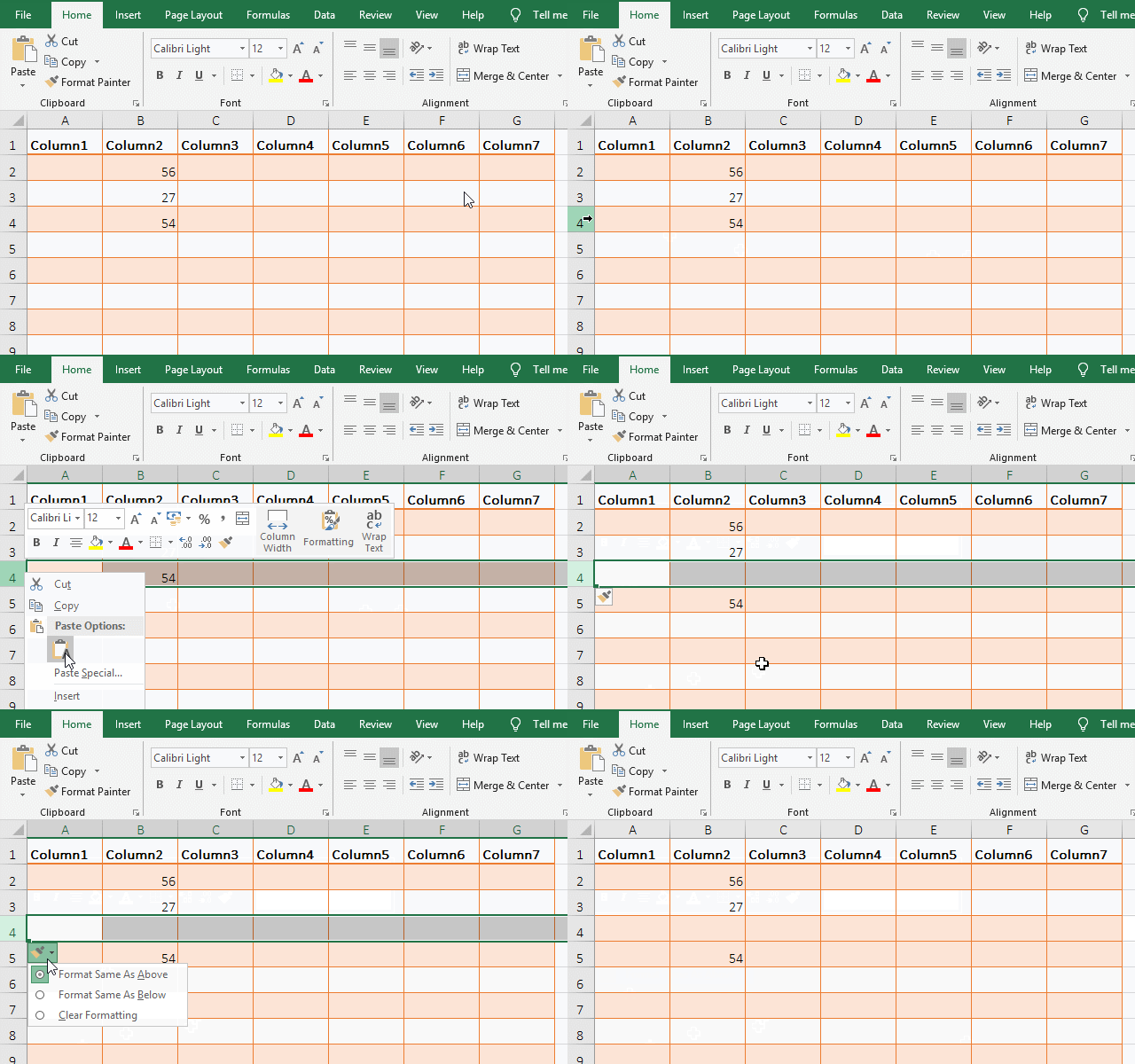
Figure 7

Tip: Press the shortcut key Alt + H + I + R to insert a row. The key method is: after selecting the position where you want to insert the row, hold down Alt and press H, I, W in order.

2. How do I insert multiple rows in excel at a time? Click the second number 2 to select the 2nd row, then click the 4th row number 4 to select the 2nd to 4th rows; right click on one of the row numbers, select "Insert" in the pop-up menu, insert three rows at a time, the original three rows are moved down; the operation process steps, see screenshot in Figure 8:

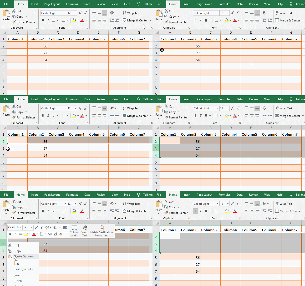
Figure 8

(II) How to insert new column in excel

1. How to insert a new column in excel? Right-click the column B of the second column, select "Insert" in the pop-up menu, insert a column in the second column, the original second column is moved to the right; click "Brush" in the upper right corner of the new column, select "Format Same As Right" in the pop-up options, the new column is the same as the format on the right, because the format of the left and right sides of the new column is the same, so can not see; the operation process steps, as shown in Figure 9:

Figure 9

Tip: Insert the column shortcut key: Alt + H + I + C, the operation method is: After selecting the position to insert the column, hold down Alt, and then press H, I, C in order.

2. How to insert multiple columns in excel at a time? Click the C of third column, hold down Shift, then click E, select the third to fifth columns; right click on one of the column numbers, select "Insert" in the pop-up menu, insert three columns at a time, the original third to fifth columns are moved to the right; the operation steps are as shown in Figure 10:

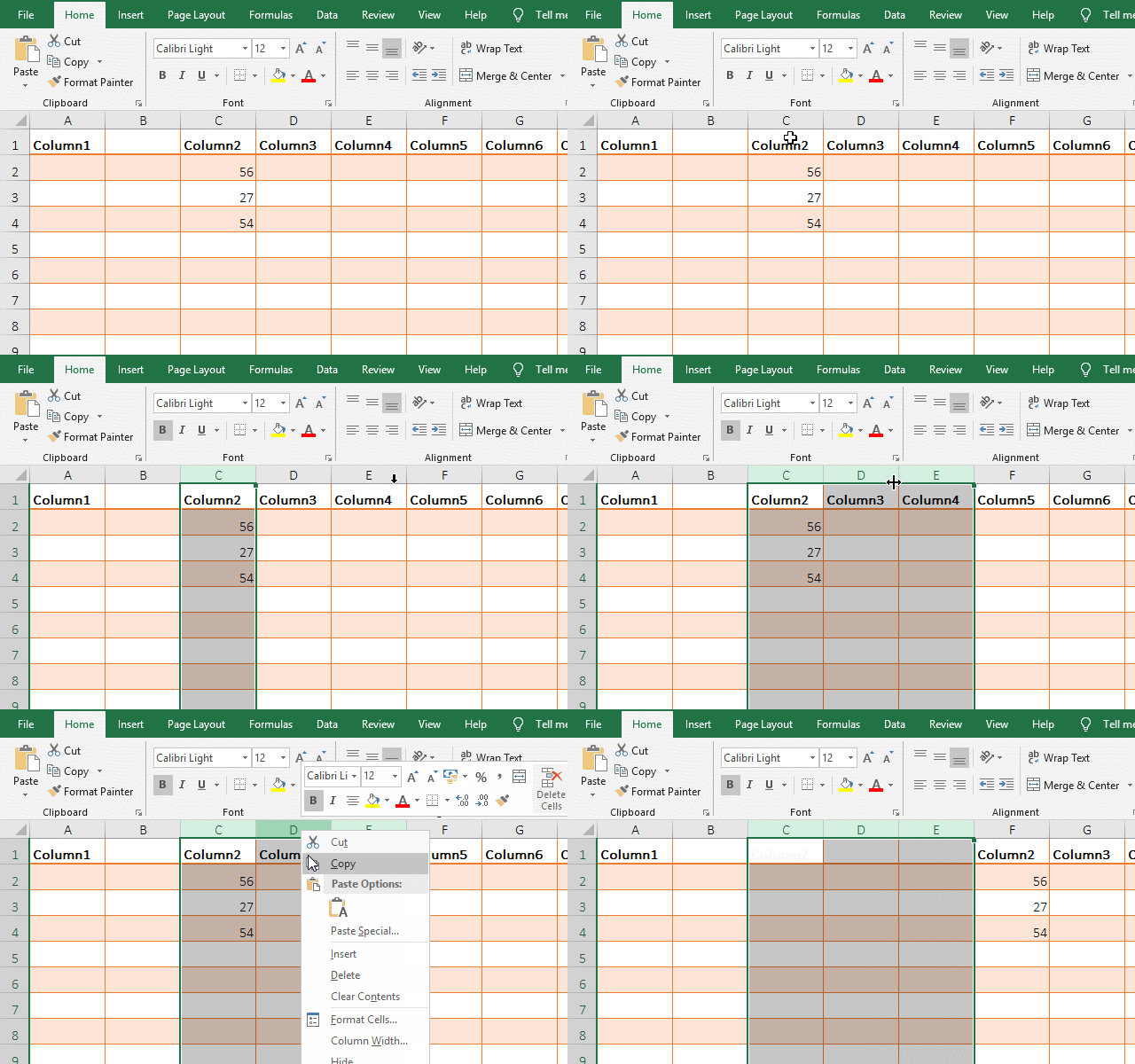
Figure 10

(III) How to insert cells in excel

1. How to insert a cell in excel? Right-click cell A2, select "Insert" in the pop-up menu, pop-up "Insert" dialog, select "Shift cells down", insert a cell in A2, the original cell is moved down; operation steps see screenshot in Figure 11:

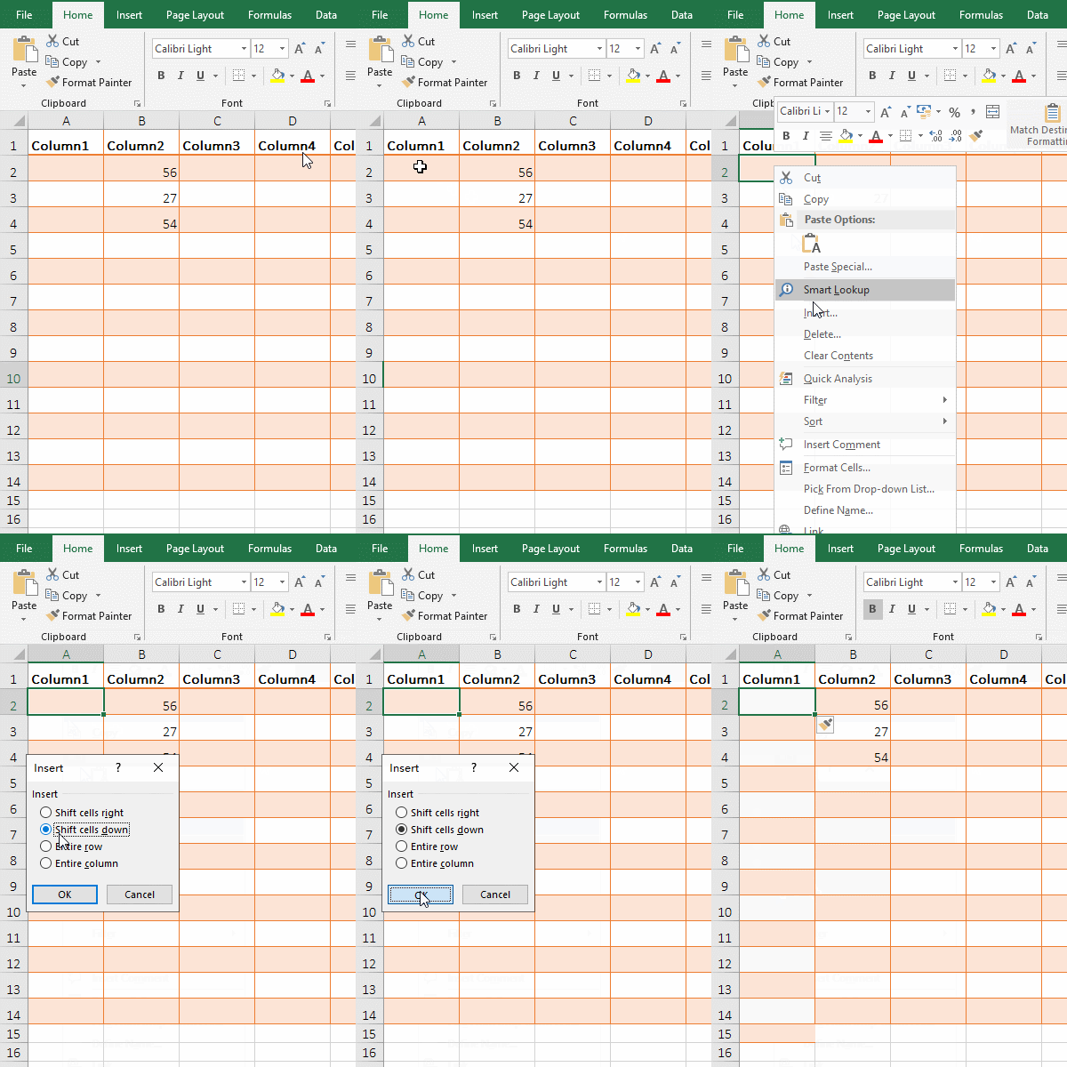
Figure 11

Tip: Insert cell shortcut key: Ctrl + Shift + = or Alt + H + I + I, the operation method is: after selecting the position of the cell to be inserted, if you use the former, press Ctrl + Shift + = at the same time; If you use the latter, hold down Alt and press H, I, I in sequence.

2. How to insert multiple cells at a time. Select the 6 cells A2:B4, right click on them, select "Insert" in the pop-up menu, pop-up "Insert" dialog, select "Shift cell right", insert 6 cells in the original 6 cells, the original cells are moved to the right; the operation steps are as shown in Figure 12:

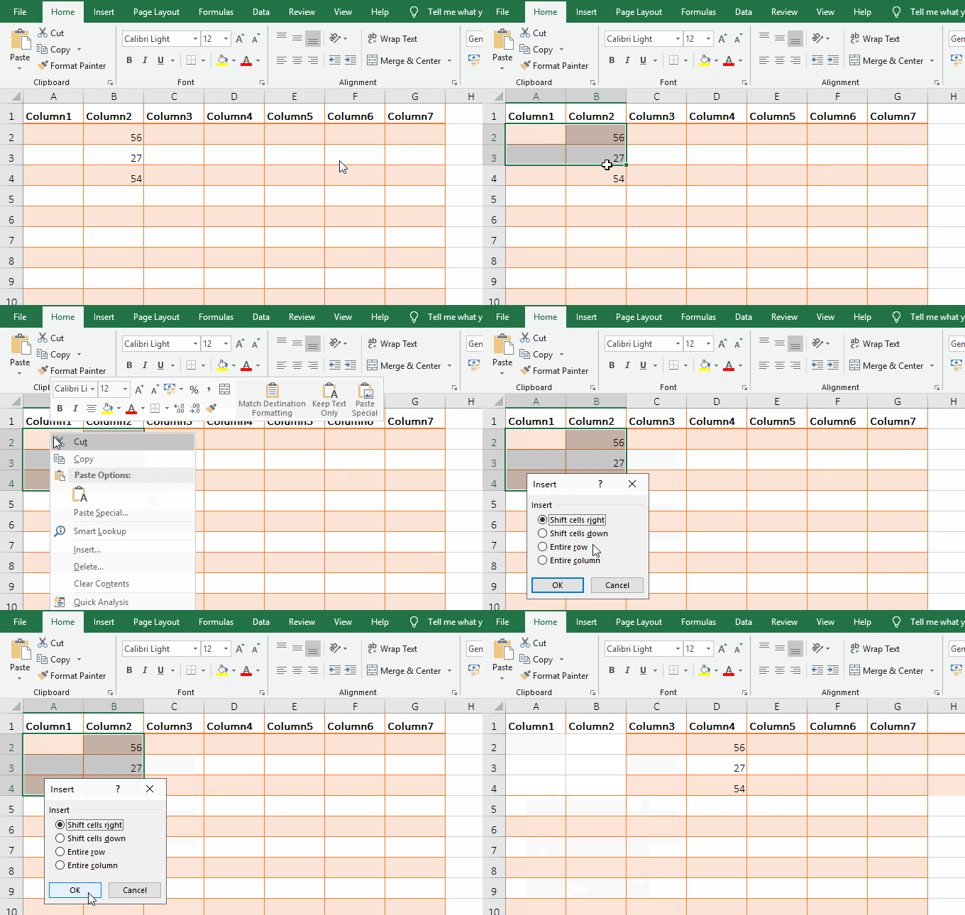
Figure 12

IV, How to delete rows, columns and cells

(I) How to delete rows in excel(delete one row or multiple rows)

Right-click the second row number 2, select "Delete" in the pop-up menu, the second row is deleted, the third row and the following rows are moved up;  click the fourth row number 4, select the second to fourth rows, right-click one of the row numbers, and select "Delete" in the pop-up menu, then the selected three rows are deleted at the same time; the operation steps are as shown in Figure 13:

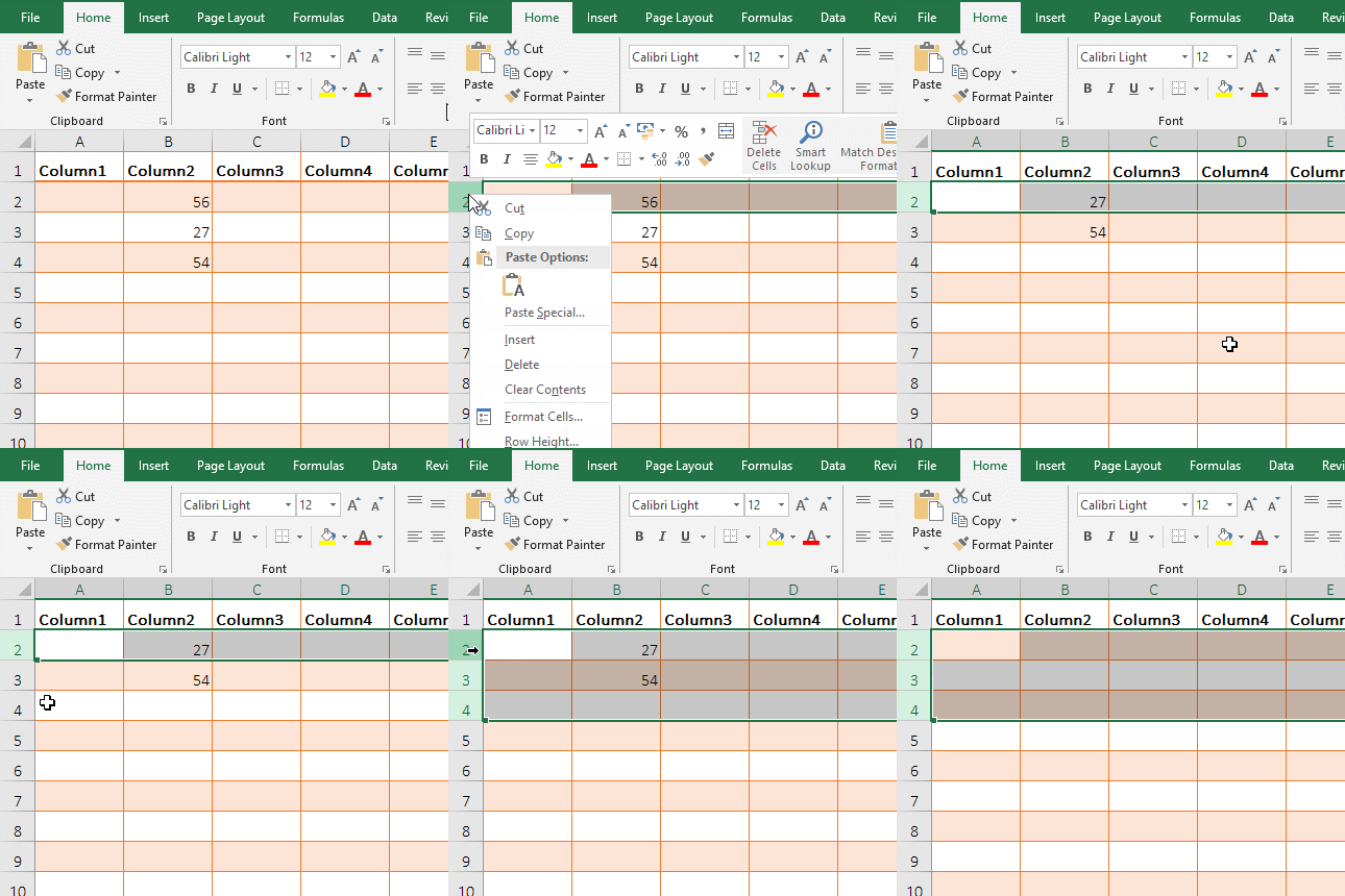
Figure 13

Tip: You can also delete the row with the shortcut key Alt + H + D + R. The operation method is: hold down Alt and press H, D, R in order.

(II) How to delete blank columns in excel(Delete one column and multiple columns)

Right click the C of third column, select "Delete" in the pop-up menu, then the third column will be deleted, the third column and following columns will be moved to the left; currently the third column is selected, hold down Shift, click the E of the fifth Column, select the third to fifth columns, right-click one of the columns, select "Delete" in the pop-up menu, the selected three columns are also deleted; the operation process steps, see screenshot in Figure 14:

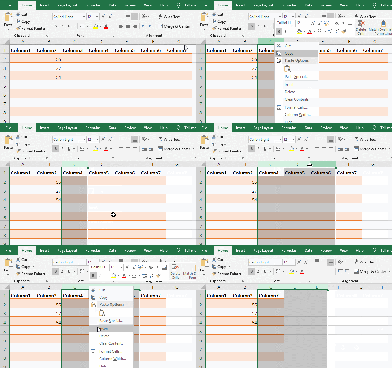
Figure 14

Tip: You can also use the shortcut key Alt + H + D + C to delete the column. The operation method is: hold down Alt and press H, D, C in order.

(III) How to delete empty cells in excel(Delete one and multiple cells)

Right-click cell B2, select "Delete" in the pop-up menu, pop-up "Delete" small dialog, select "Shift cells left", then B2 will be deleted, and the cells on the right will be moved to the left to supplement it; Select the six cells B2:C4, right click on them, select "Delete" in the pop-up menu, then the selected six cells will be deleted at the same time; the operation steps are as shown in Figure 15:

Figure 15

Tip: You can also use the shortcut key Alt + H + D + D to delete the cell. The operation method is: hold down Alt and press H, D, D in order.

V, How to move rows, columns and cells

1. How to move a row or multiple rows in excel

A. How to move a row in excel? Select the second row, move the mouse to the lower line of the second row, hold down Shift and left button of mouse, drag down and drag to the position you want to move, such as row 4, when the bottom line of the 4th row appears bold green lines, release the left button, the second row is moved to the 4th row, and the second and third rows are moved up; see screenshot in Figure 16.

B. How to move multiple rows in excel? The 4th row is currently selected, click the second row, the second to fifth rows are selected, and move the mouse to the on the lower line of the four rows, hold Shift and the left button of mouse and move down to the 7th row, when the lower line of the 7th row appears the bold lines, release the left button, then the selected three rows are moved down three rows; the process steps are shown in Figure 16:

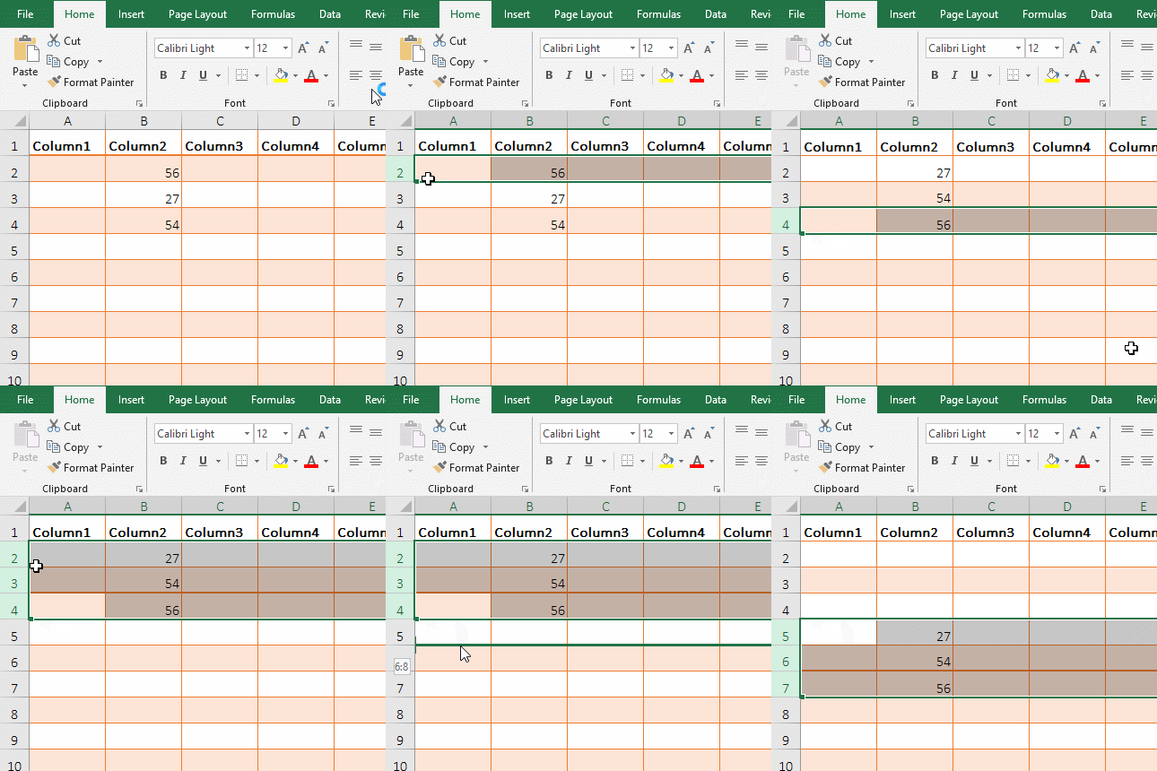
Figure 16

2. How to move columns in excel

Click B to select the second column, move the mouse to the right line of the second column, hold down Shift and the left button of mouse, drag to the right and drag to the D column, when the right line of the D column appears the bold green lines, release the left key of mouse, the second column is moved to the fourth column, the operation steps, see screenshot in Figure 17:

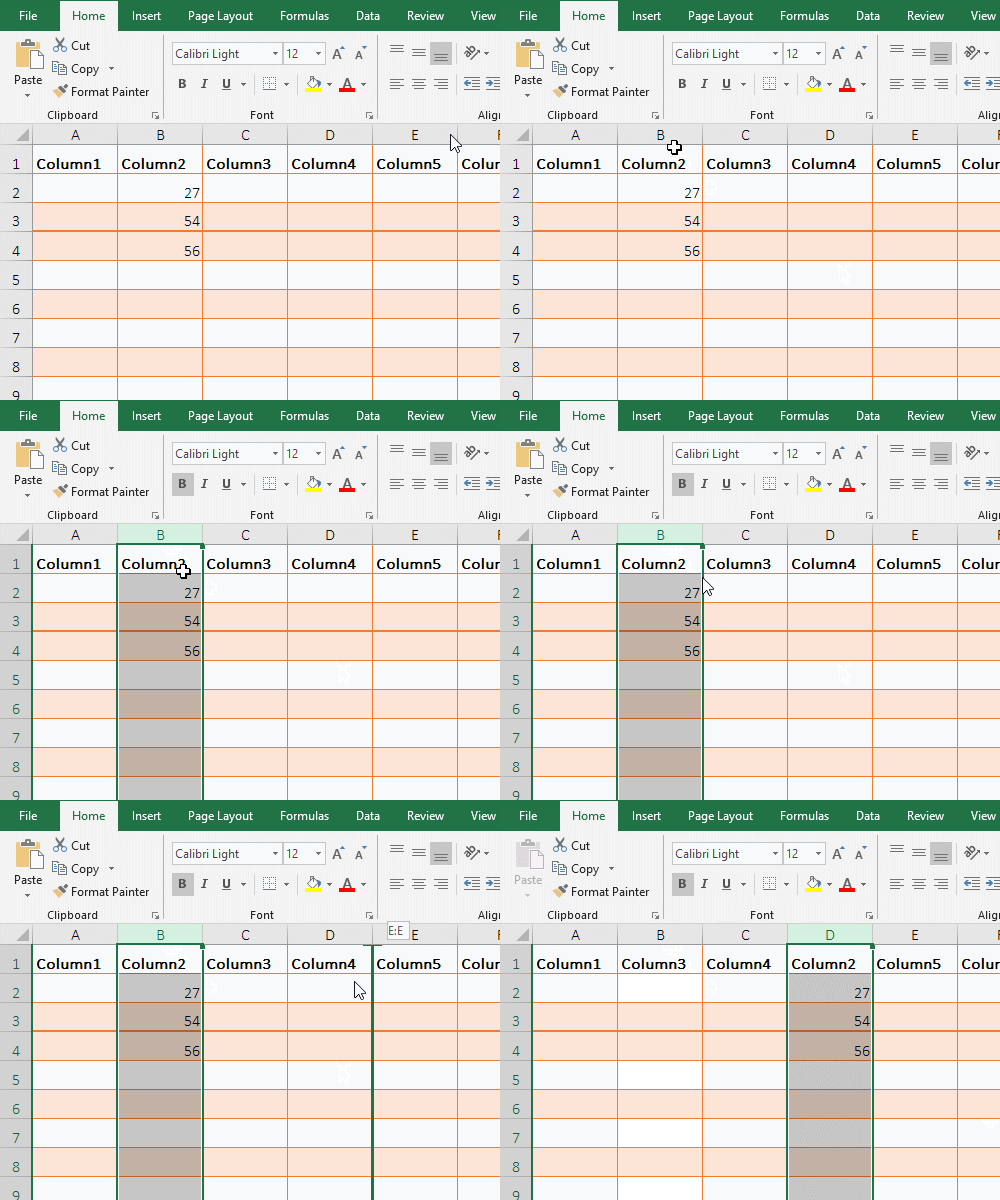
Figure 17

3. How to move one and more cells

Click B2 to select it, move the mouse to the right line of B2, hold down Shift and left button of mouse, drag to the right and drag it to D4, when D4 has a bold green I-word on the right line, release the left button, B2 is moved to D4; select B3:B4, move the mouse to the lower line of B4, hold down Shift and left button of mouse, move down until to B7, when B7 appears a green I-word, release the left button, then B3:B4 is moved to B6:B7; the operation steps are as shown in Figure 18:

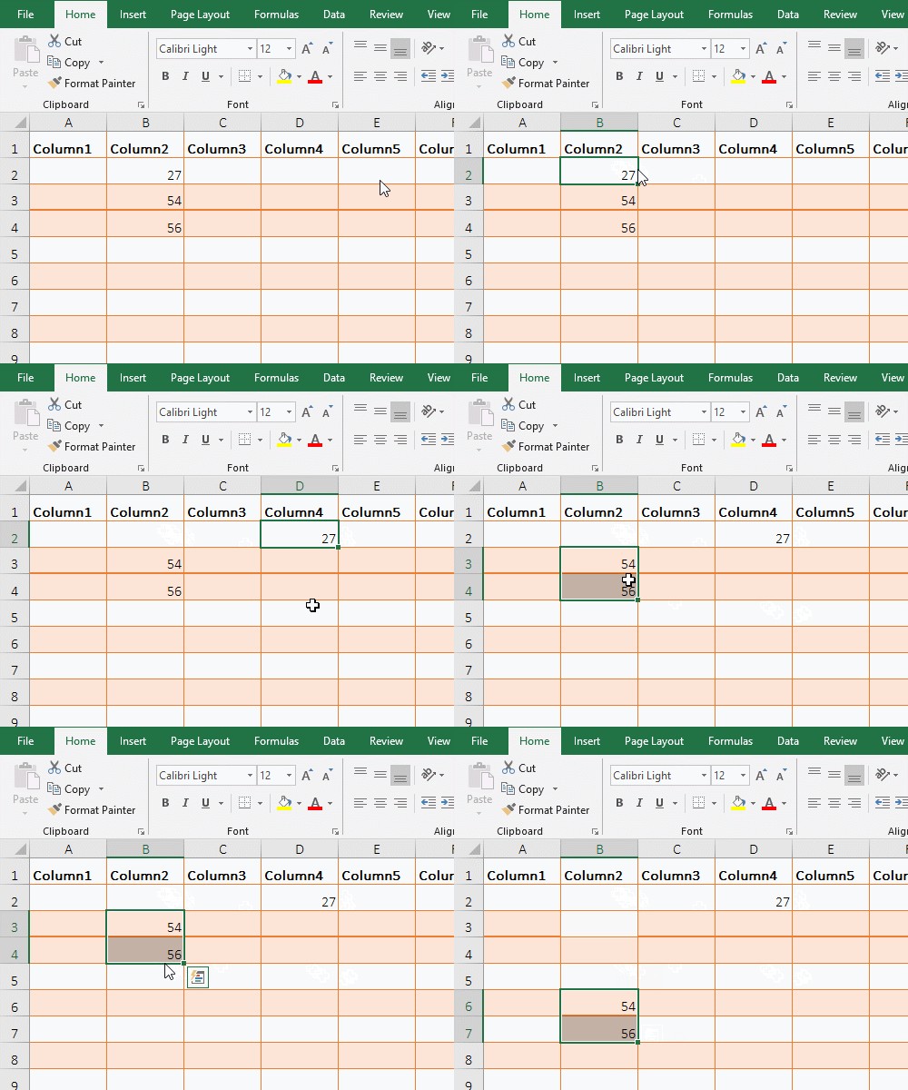
Figure 18

VI, Table text editing

(I) How do you wrap text in excel

1. If you want to enter the "White long sleeve shirt" in cell A1. Click A1 to select it, enter the "White long", the text has already filled the cell, press the shortcut key Alt + Enter to change the line, continue to enter "sleeve shirt", the operation process steps, see screenshot in Figure 19:

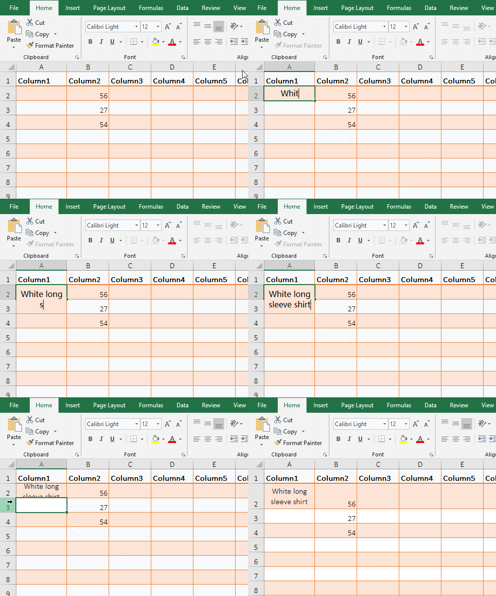
Figure 19

Tip: After pressing Alt + Enter twice, Excel will remember the wrap operation. If you continue to enter, when the text exceeds one line, it will automatically wrap.

2. Add data to the table with the method above, of course, if you has prepared the data in the computer and is in the form of a table, you can also copy it to the Excel table at one time.

(II) How to add title to excel spreadsheet

Right-click the first row number 1, select "Insert" in the pop-up menu, insert a row in the first row; pull the first row high, Select cell A1, enter the spreadsheet name "Clothes Sales", press Enter to exit input; select A1:G1, the current tab is "Home", click "Merge & Center", the selected seven cells are merged into one; click the "Middle Align" icon, center the text vertically; click the "Font" drop-down list box, select a font, such as "Arial Black"; click the "Font Size" drop-down list box, select a font size, for example 22; click the down arrow to the right of "Font Color", select one of the pop-up color styles, such as "Orange, Accent 2", the title of spreadsheet is created, the operation steps, as shown in Figure 20:

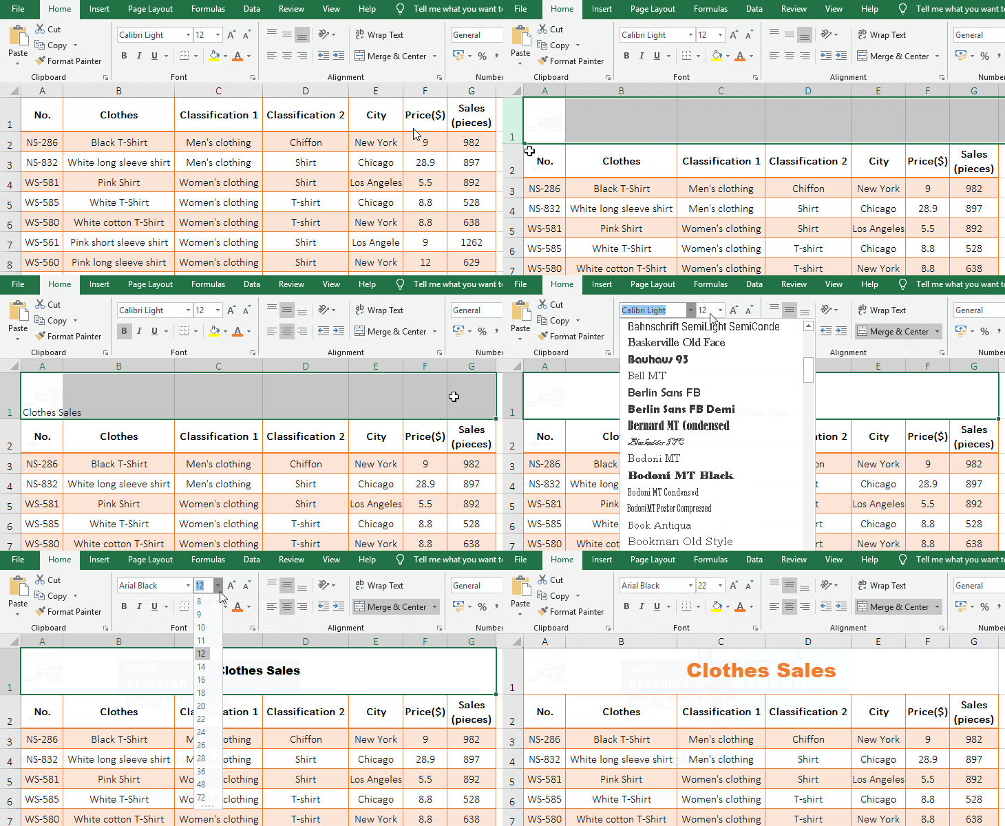
Figure 20

VII, How to format cells in excel

1. How to change alignment in excel

Click A to select the first column, hold down the Shift key, click the letter G in the last column, select all the columns in the table, the current tab is "Home", click the "Center" icon, then all the columns are centered; select F1:G1, press and hold Alt, press H once, press W once, the words in F1 and G1 will automatically wrap; the operation steps are as shown in Figure 21:

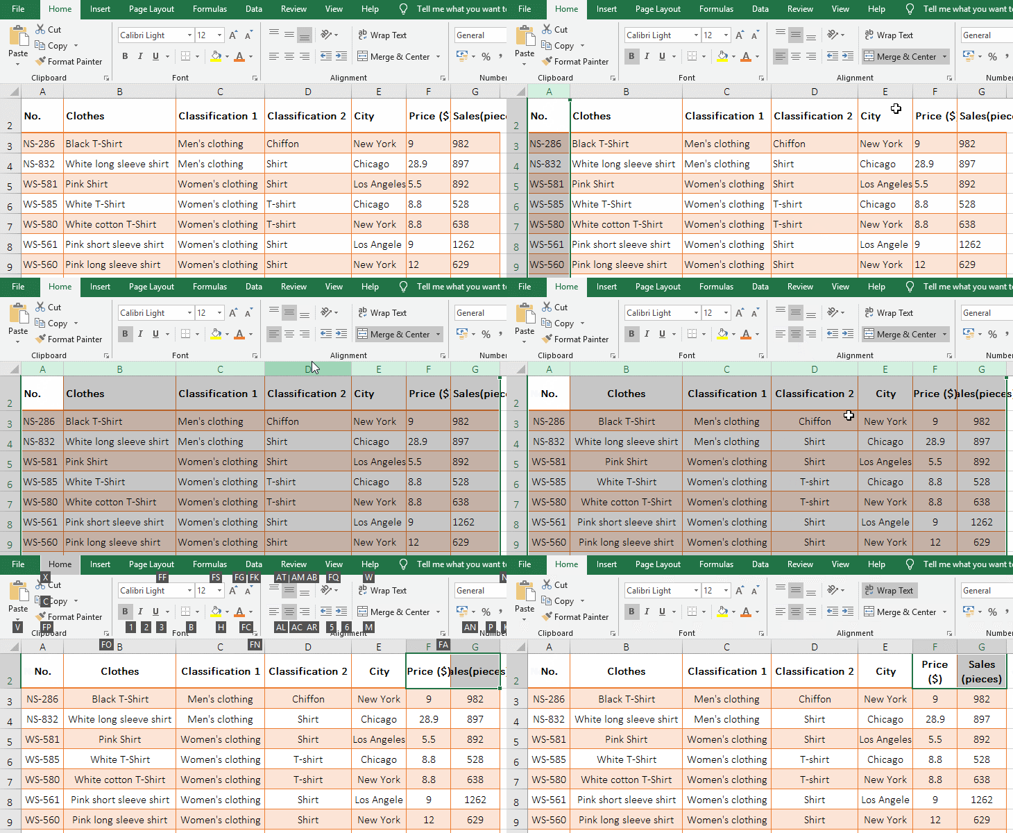
Figure 21

2. How to set the cell background and how to change font color in excel

 Select A1:G1, the current tab is "Home", click the "Fill Color" icon to the right of the down arrow, select "Orange, Assent 2, Lighter 80%" in the pop-up color style, then the texts in the first row are changes to the selected color; click the down arrow to the right of the "Font Color" icon, select "Orange, Assent 2", then the selected texts become the selected color; the operation steps are as shown in Figure 22:

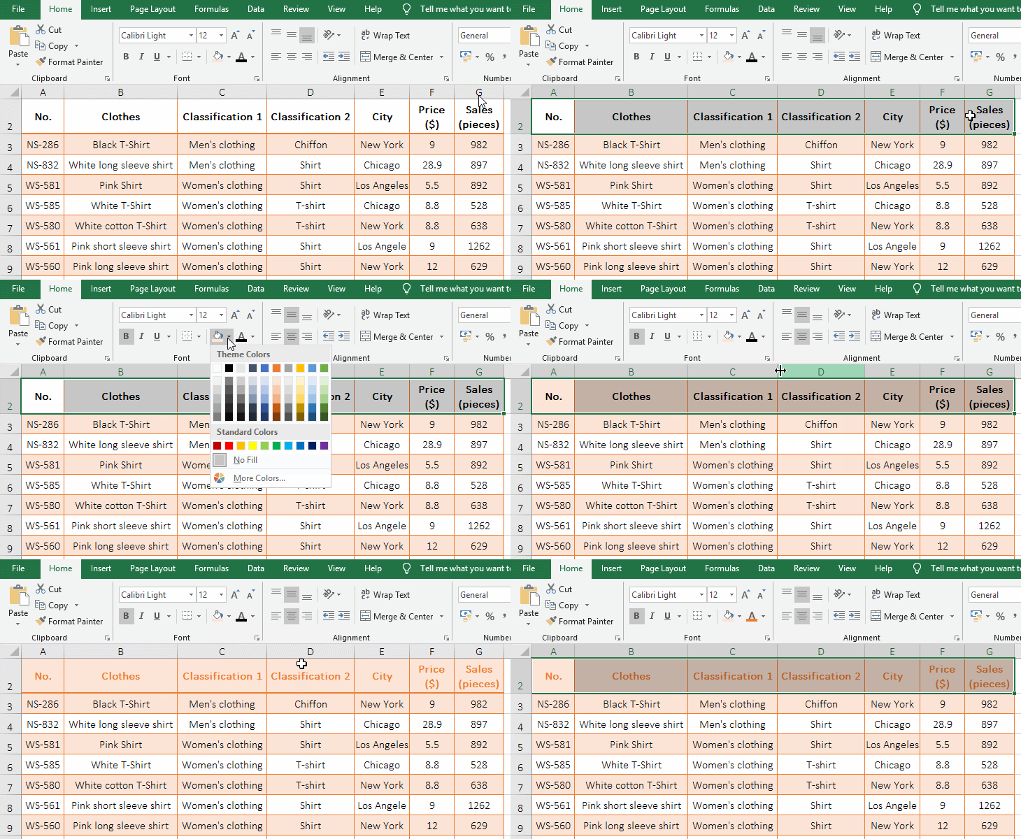
Figure 22

Tip: If you want to set the font or font size for the text, click the "Font or Font Size" drop-down list box to select or click the "Increase Font Size or Decrease Font Size" icon; if you want to set the text to bold, italic and underline, Click on these icons.

3. Select cell style

Select A1:G1, the current tab is "Home", click "Cell Styles", expand a variety of cell styles that are built-in excel, you can select while previewing, if you find the appropriate, click, we choose "Light Orange, 60% - Accent 2", the selected style is applied to all cells in the first row; the operation steps are as shown in Figure 23:

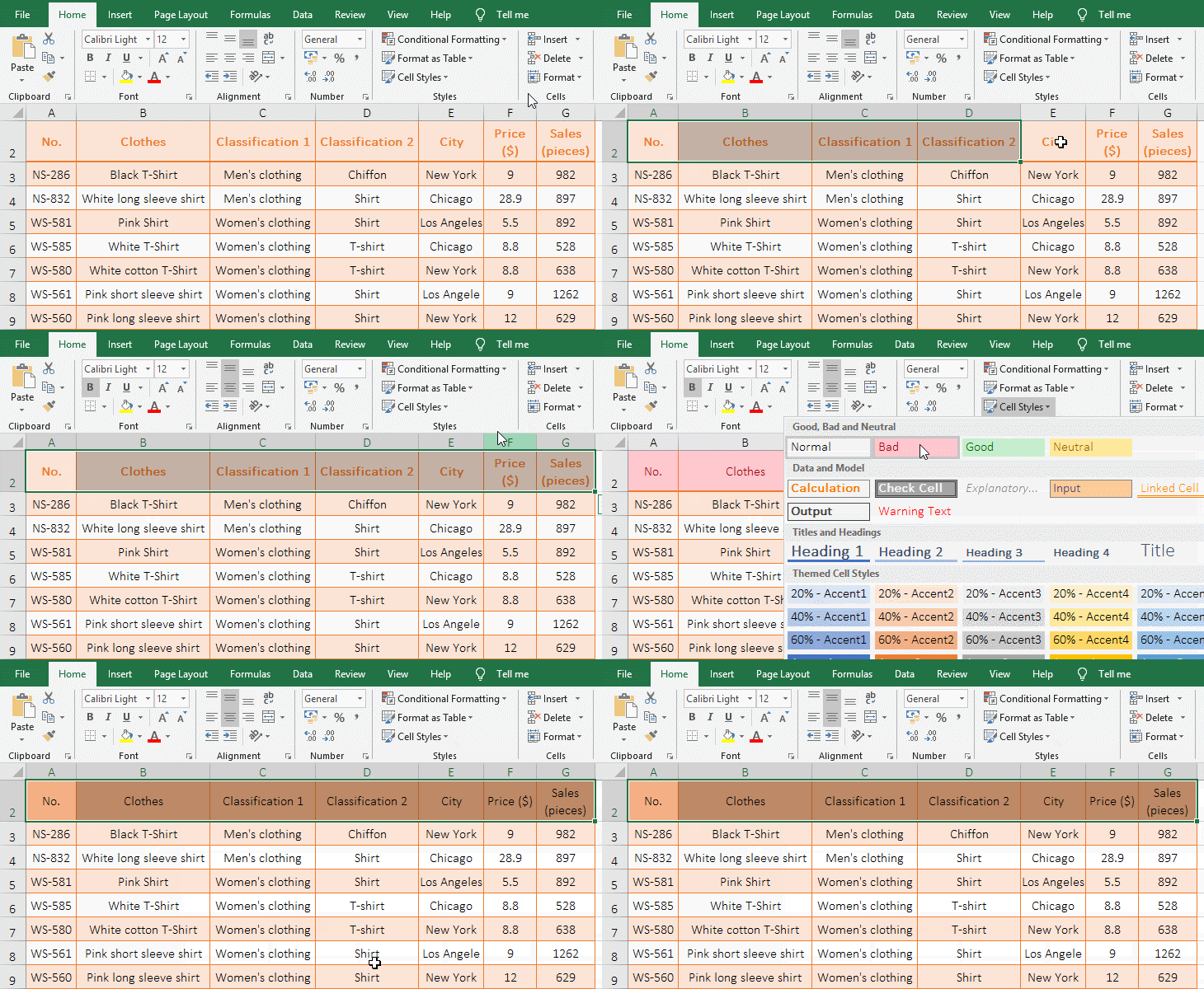
Figure 23

VIII, How to add borders in excel

1. How to add border for table

Click A1 to select it, hold down the Shift key, click G15 to select the entire table, press the shortcut key Ctrl + 1, open the "Format Cells" dialog, select the "Border" tab, click color drop down list, select "Orange, Accent 2, Lighter 40%" in the pop-up color style; "Line Style" keeps the default, then select the "Outline and Inside" icons under "Presets", click "OK", then set the border to apply to the table; the operation process steps, as shown in Figure 24:

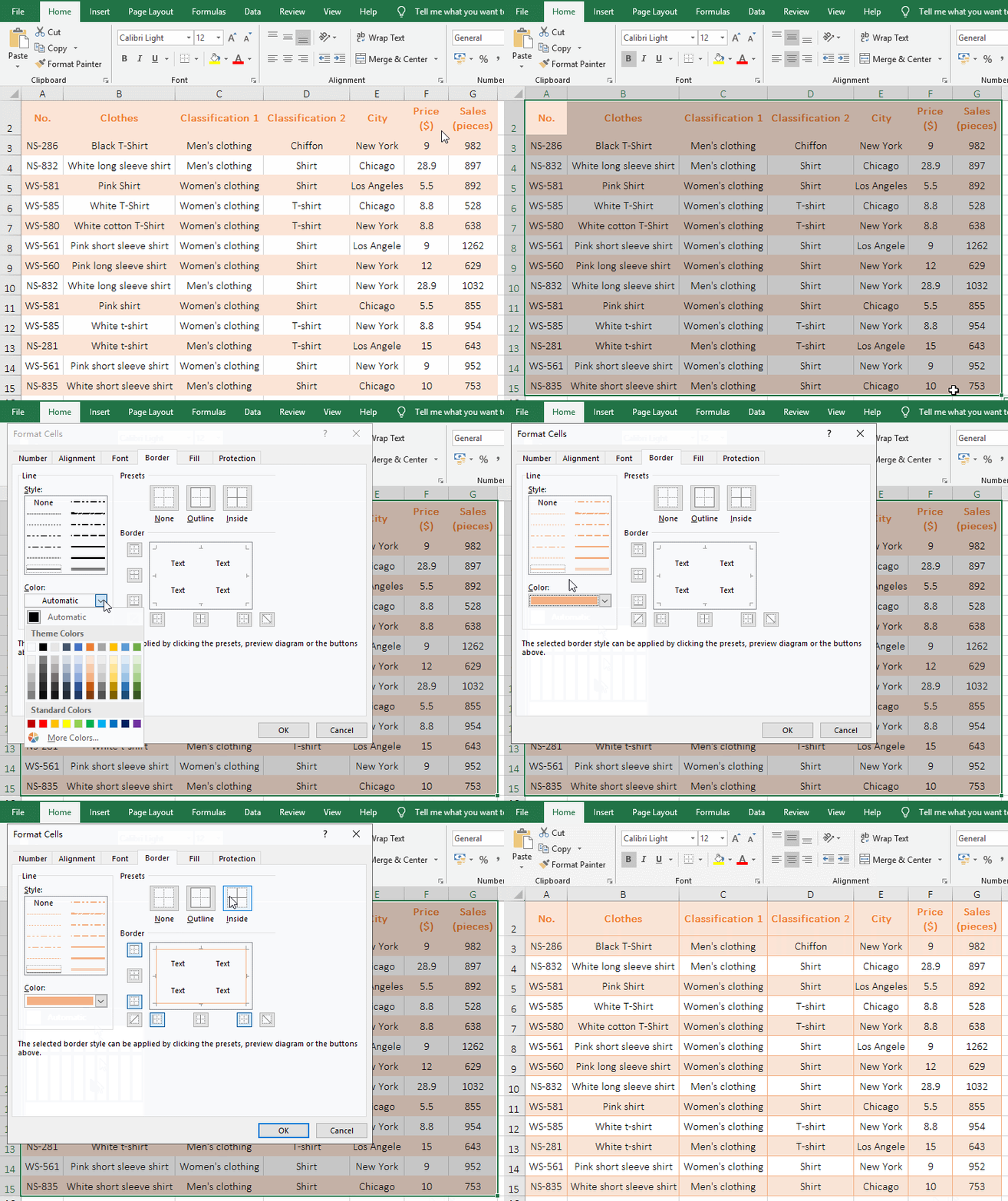
Figure 24

2. How to add cell borders in excel

The table has three cells (B4, B6 and C5) that have no borders, and you want to set them to the same border as the other cells. Select B4, hold down Ctrl, click B6 and C5 respectively, select three cells; press Ctrl + 1, open the "Format Cells" dialog, select the "Border" tab, click color drop down list, select "Orange, Accent 2, Lighter 40%" in the pop-up color style; select "Outline" icon under "Presets", click "OK", then the three cells are added with the same border as the other cells of the table; the operation process steps are as shown in Figure 25:

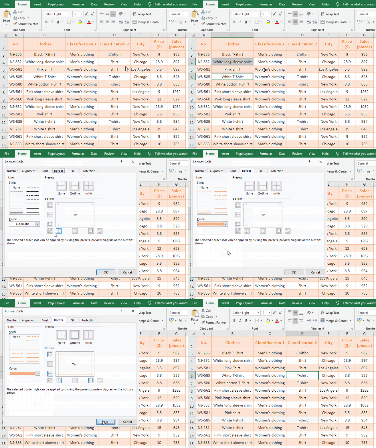
Figure 25

IX, Sum

1. How do I sum a column in excel

If you want the sum of clothing sales. Select cell G16, press the sum shortcut Alt + =, then the sum formula =SUM(G3:G15) is automatically input to G16, press Enter to find the sum of the clothing sales; the operation steps are as shown in Figure 26:

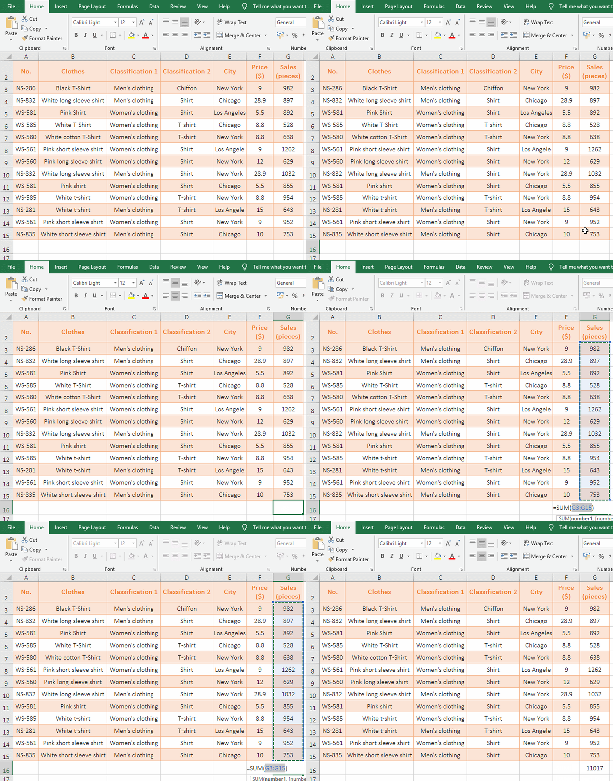
Figure 26

2. How to sum rows in excel

If you want the sum of sales of each type of clothing every month. Select cell F2, press Alt + =, then the sum formula =SUM(B2:E2) is automatically input to F2, press Enter to find the sales volume of all kinds of clothing in January; move the mouse to cell fill handle in the lower right corner of F2, double-click the left button to find the sales volume of all kinds of clothing in the remaining months; the operation process steps, as shown in Figure 27:

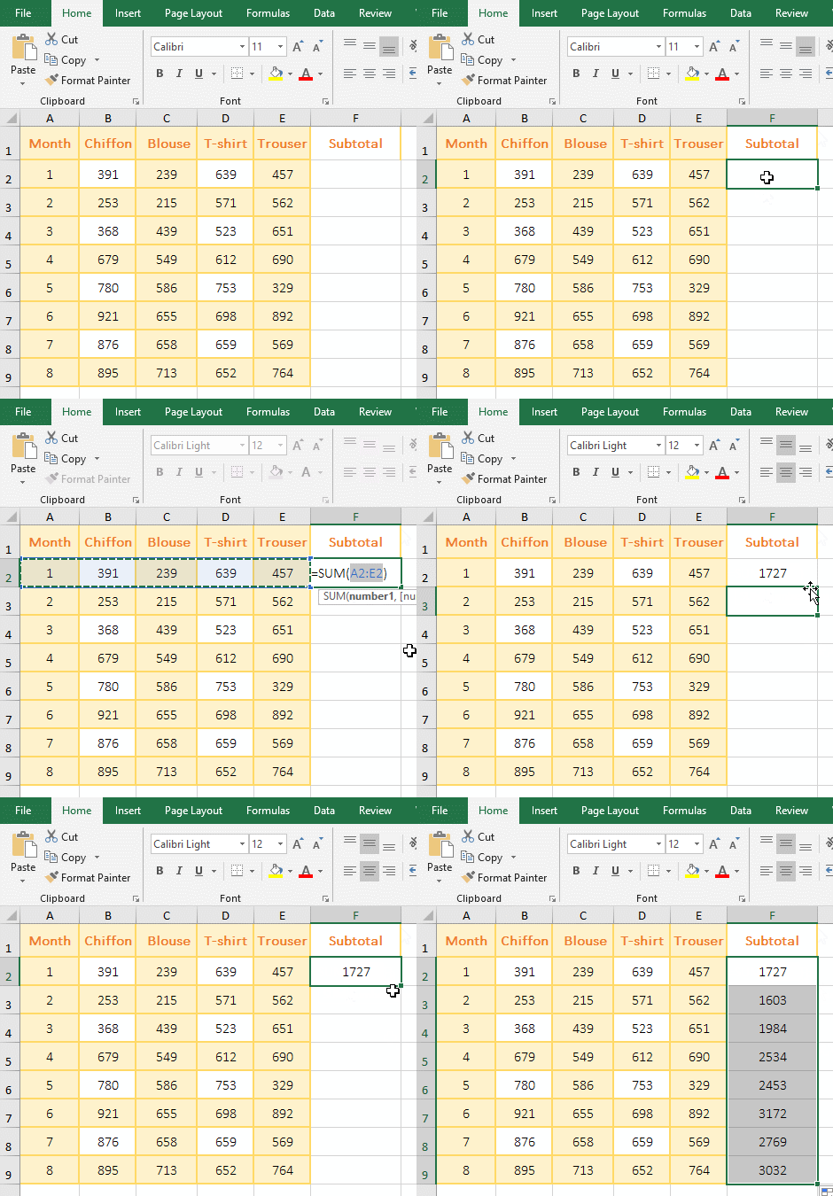
Figure 27

X, Average

If the average price of clothing is required. Select cell F16, select the "Formulas" tab, click the down arrow under "AutoSum", select "Average" in the pop-up menu, then average the formula = AVERAGE(F3:F15) is automatically inputted to the F16 and press Enter to return the average price of 12.24615385
; select F16 again, press Ctrl + 1, open the "Format Cells" dialog, select the "Number" on the left, and the "Decimal Places" keep the default two digits. Click "OK", the average price becomes 12.25; the operation process steps, see screenshot in Figure 28:

Figure 28