How to use Excel rank function(11 examples, with Rank.EQ and Rank.AVG, without skipping numbers)

The Rank function is used to return the rank of the specified number in the list of numbers in Excel. Applying this function allows you to sort or rank the list of numbers in ascending or descending order. The Rank function has been replaced with the Rank.EQ function and the Rank.AVG function In the new version of Excel.

The Rank function ranks duplicate numbers side by side with a repeating number and leaves an interval. If the number after the repeated number is required to follow the repeated number ranking, you need to use Sum + If + CountIf, SumProduct + CountIf or Sum + If + FreQuency. The following are 11 examples of how to use the Rank function, including the basic usage of the Rank function, the difference between Rank and Rank.EQ, Rank.AVG, side by side or sequential automatic ranking with repeated numbers, segmentation sorting, sorting the number list to the row and rank duplicates without skipping numbers

I, Excel Rank function syntax

1. Expression: RANK(Number,Ref,[Order])

2. Description:

A. Ref is a reference to an array or range of cells containing a list of numbers; if there are non-numeric values in Ref, they are ignored.

B. Order is optional, it is used to specify the ranking of the number; if Order is omitted or 0, the number list are sorted in descending order  by the Rank function; if Order is non-zero, the list of numbers are sorted in ascending order by the Rank function.

C. If there are the duplicate numbers in the list of numbers, how do they rank? See "How to use the Excel Rank function ."

II, The difference between Excel Rank, Rank.EQ and Rank.AVG function

The Rank.EQ and Rank.AVG function are used to replace the Rank function. The differences are as follows:

1. Rank.EQ has the same function as Rank, ie Rank.EQ inherits all the functions of Rank. The expression of Rank.EQ is as follows:

RANK.EQ(Number,Ref,[Order])

2. The difference between Rank.AVG and Rank(Rank.EQ) is mainly in the ranking of the same number; Rank.AVG returns the average ranking for the same number, and Rank(Rank.EQ) returns the best ranking, ie, juxtaposition Sort. The expression for Rank.AVG is:

RANK.AVG(Number,Ref,[Order])

III, How to use the Excel Rank function(how to use the Rank.EQ in excel)

(I) How to rank numbers in excel

1. If you want to return the rank of sales volume 1850 in descending order or in ascending order. Double-click cell D8, copy the formula =RANK(1850,D2:D7) to D8, press Enter, return to 6; double-click D9, copy the same formula to D9, then enter ",1" after D2:D7, press Enter, return 6; the operation steps, as shown in Figure 1:

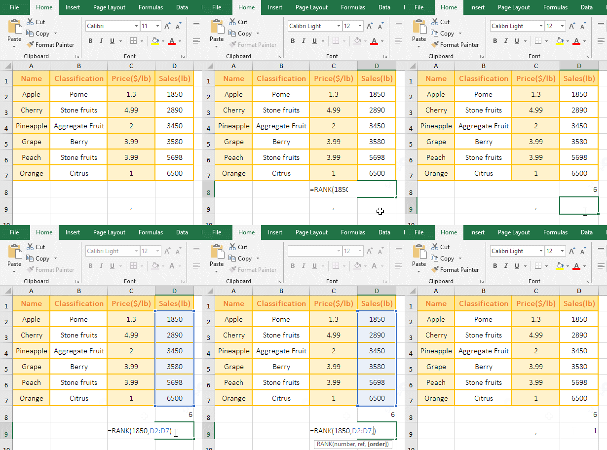
Figure 1

2. Description:

A. 1850 is the Number to be ranked, D2:D7 is the Ref in the formula =RANK(1850,D2:D7), the formula omits the argument Order, D2:D7 is ranked by default in descending order; the rank of 1850 returnted in D2:D7 is 6, which is the result of D2:D7 ranked in descending order.

B. The Order is set to 1 in the formula =RANK(1850,D2:D7,1), then 1850 is ranked in ascending order in D2:D7.

(II) Automatic sorting examples without duplicate numbers

1. If you want to rank sales in descending order. Double-click cell E2, copy the formula =RANK(D2,D$2:D$7) to E2, press Enter, return 6; select E2, move the mouse to the cell fill handle in the lower right corner of E2, after the mouse becomes bold black plus, double-click the left button to return the ranking of the remaining values, and the sales column is also ranked in descending order; the operation steps are as shown in Figure 2:

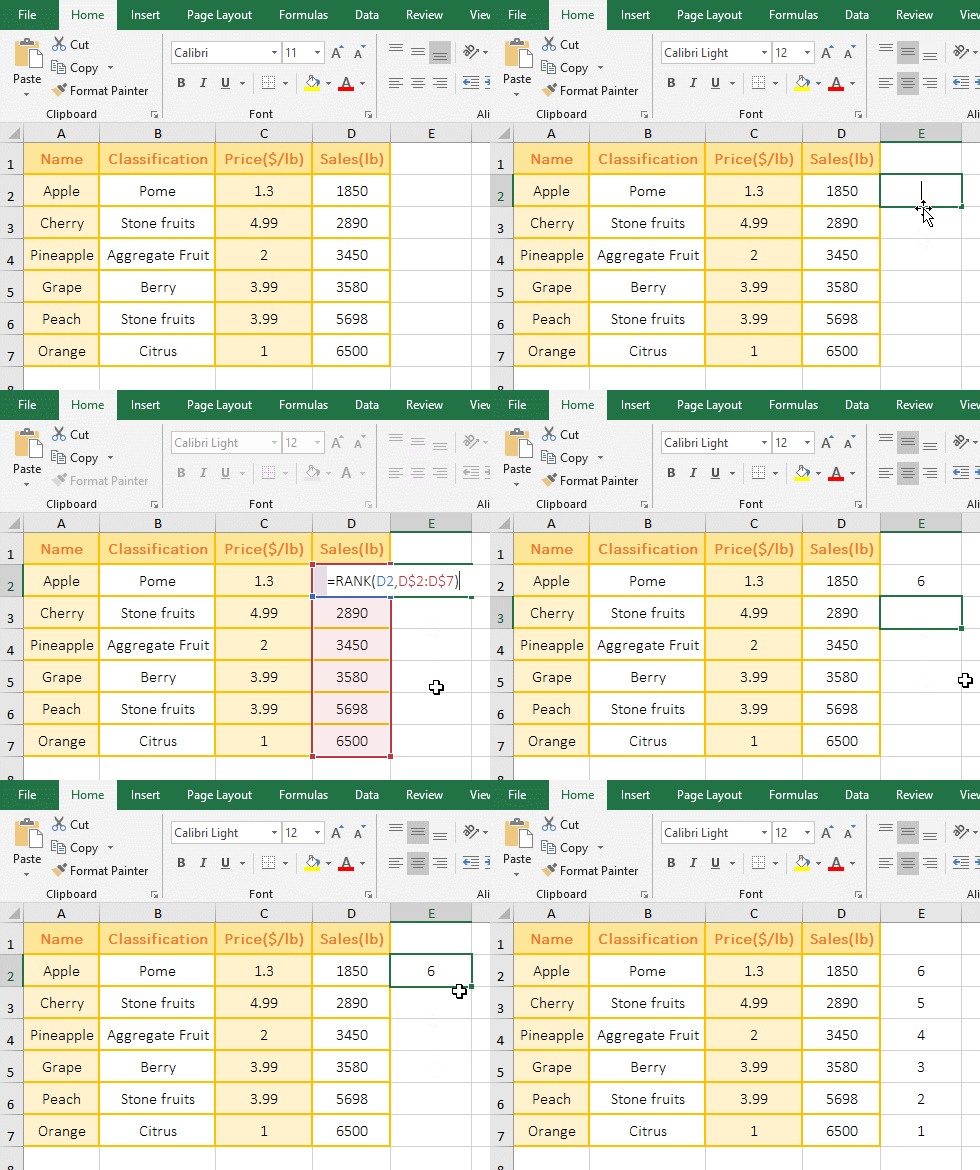
Figure 2

2. Formula =RANK(D2,D$2:D$7) description:

A. D2 are relative references to columns and rows. When dragging down, D2 will become D3, D4, etc.; $ means absolute reference to the row in D$2:D$7, when dragging down, D$2 will not becomes D3, D4, etc., and D$7 is the same as D$2.

B. When the formula is in D2, it returns to the rank 6 of the number in D2 in D2:D7; when the formula is in D3, it returns to the rank 5 of the number in D3 in D2:D7; the others and so on.

(III) Duplicate numbers are automatically ranked side by side

1. If you want to rank the price in ascending order. Double-click cell E2, copy the formula =RANK(C2,C$2:C$7,1) to E2, press Enter, return to 2; select E2, and double-click the cell fill handle to return the rank of the remaining value, the price column is also ranked accordingly; the operational steps are shown in Figure 3:

Figure 3

2. Formula =RANK(C2,C$2:C$7,1) explanation:

A. The formula = RANK(C2,C$2:C$7,1) and the formula of the above example =RANK(D2,D$2:D$7) is a meaning, but here the argument Order is set to 1, that is, C2:C7 Ascending.

B. There is a repeating number 3.99 in C2:C7, both of which are ranked 4th, indicating that the Rank function puts the repeated numbers side by side.

(IV) Duplicate numbers are ranked in ascending order automatically

1. Also take the example of ranking the price in ascending order. Double-click cell E2, copy the formula =RANK(C2,C$2:C$7,1)+COUNTIF(C$2:C2,C2)-1 to E2, press Enter, return to 2; select E2, also double-click the cell fill handle to return the rank of the remaining values, and the price column is also ranked in ascending order; the operation steps are as shown in Figure 4:

Figure 4

2. Formula =RANK(C2,C$2:C$7,1)+COUNTIF(C$2:C2,C2)-1 explanation:

A. C$2:C2 is used to return the value of C2 to C2. When dragging down, C2 will change to C3, C4, etc., and C$2 will not change, which will realize statistics of the number from C2 to the dragged to cell. So how are the duplicate numbers sorted in ascending order by CountIf function?

B. When the formula is in E2, COUNTIF(C$2:C2,C2) counts the number of C2(ie 1.3) in C2, and the result is 1; RANK(C2,C$2:C$7,1) returns the rank 2 of C2 in C2:C7, 2 + 1 - 1 is exactly equal to 2.

C. When the formula is in E3, COUNTIF(C$2:C3,C3) counts the number of C3(ie 4.99) in C2:C3, and the result is also 1; RANK(C3,C$2:C$7,1) returns the rank 6 of C3 in C2:C7, 6 + 1 - 1 is exactly equal to 6.

D. When the formula is in E6, COUNTIF(C$2:C6,C6) counts the number of C6 in C2:C6, the result is 2(C2:C6 has two 3.99), and RANK(C6,C$2:C$7 , 1) returns the rank 4 of C6 in C2:C7, 4 + 2 - 1 is exactly equal to 5; thus the duplicate numbers 3.99 is ranked (one ranks 4, the other ranks 5).

IV, The difference between Excel Rank function(Rank.EQ function) and Rank.AVG function

(I) Returning the ranking of duplicate numbers

1. If you use three functions to return the ranks of 3.99 in the "Price". Double-click cell E2, copy the formula =RANK(3.99,C2:C7) to E2, press Enter, return 2; double-click F2, copy the formula =RANK.EQ(3.99,C2:C7) to F2, press Enter, also returns 2; double-click G2, copy the formula =RANK.AVG(3.99,C2:C7) to G2, press Enter, return to 2.5; the operation steps, as shown in Figure 5:

Figure 5

2. Formula description:

As you can see from the demo, the Rank function returns the same result as the Rank.EQ function, and the Rank.AVG function returns 2.5. How did this 2.5 come from? There are two 3.99 in C2:C7, one 3.99 ranks in the 2nd position, the other 3.99 ranks in the 3rd position in descending order, Rank.AVG returns the average rank of the same value, and the average of 2 and 3 is 2.5. Therefore, the rank of 3.99 is 2.5.

(II) Duplicate numbers are automatically ranked

1. If you use three functions to rank the "price" in descending order. Double-click cell E2, copy the formula =RANK(C2,C$2:C$7) to E2, press Enter, return 5; returns the ranking of the remaining price with double-clicking the cell fill handle. Double-click F2, copy the formula =RANK.EQ(C2,C$2:C$7) to F2, press Enter, return 5, return the ranking of the remaining price in the same way; then copy the formula =RANK.AVG(C2,C$2:C$7) to G2, press Enter, return to 5, and return the ranking of the remaining price in the same way; the operation steps are as shown in Figure 6:

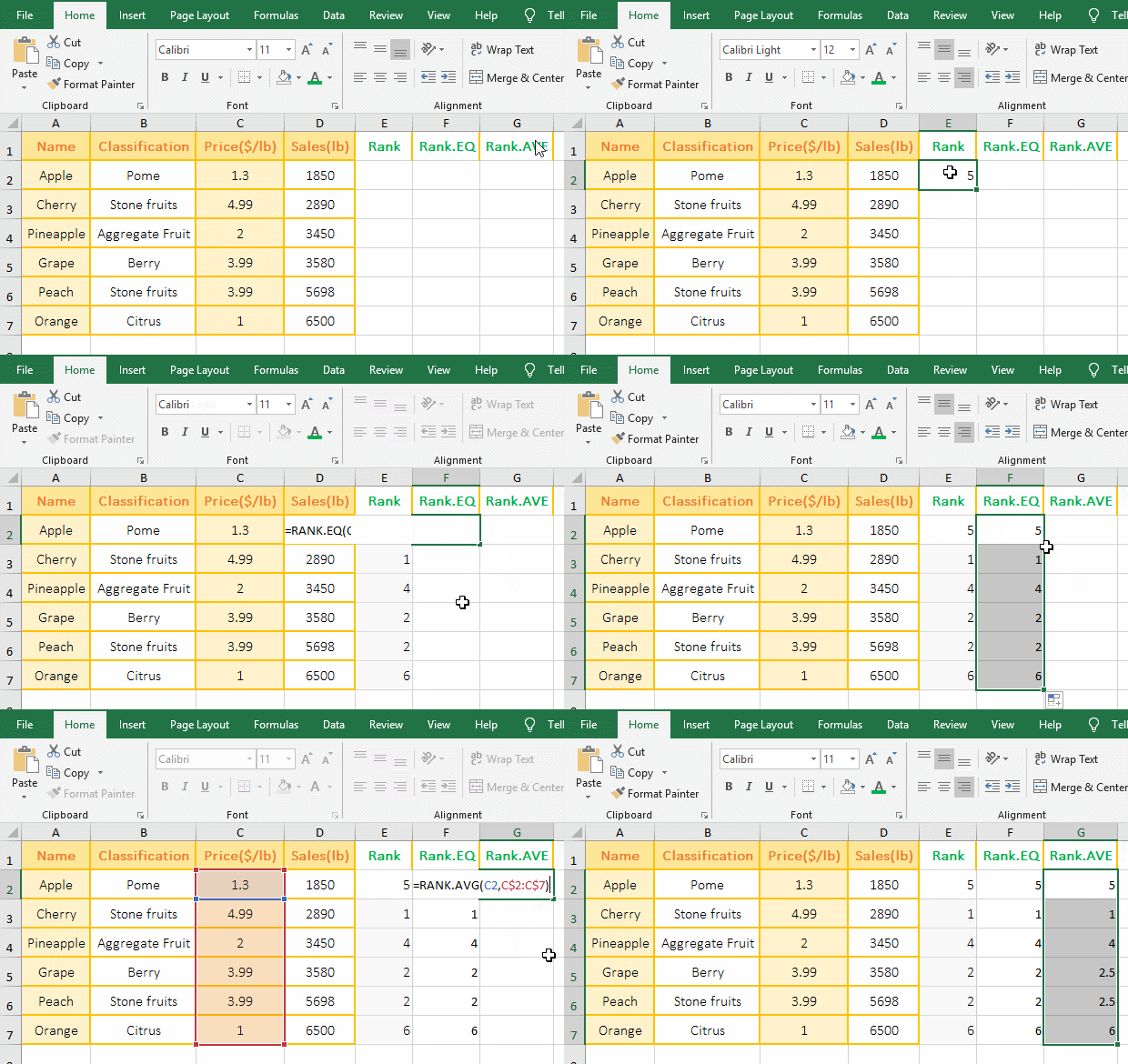
Figure 6

2. Formula description:

As can be seen from the demo, the Rank function is exactly the same as the Rank.EQ function, and the Rank.AVG function takes the average ranking for duplicate numbers, both of which are ranked 2.5.

V, The extended application examples of Excel Rank function

(I) Rank + OffSet + Row combination for segmentation ranking

1. If it is required to rank the sales by quarter. Double-click cell C2, copy the formula =RANK(B2,OFFSET(B$2:B$4,INT((ROW()-2)/3)*3,),1) to C2, press Enter, return 2; Select C2, returns the rank of other numbers with the method of double-clicking the cell fill handle; the operation steps are as shown in Figure 7:

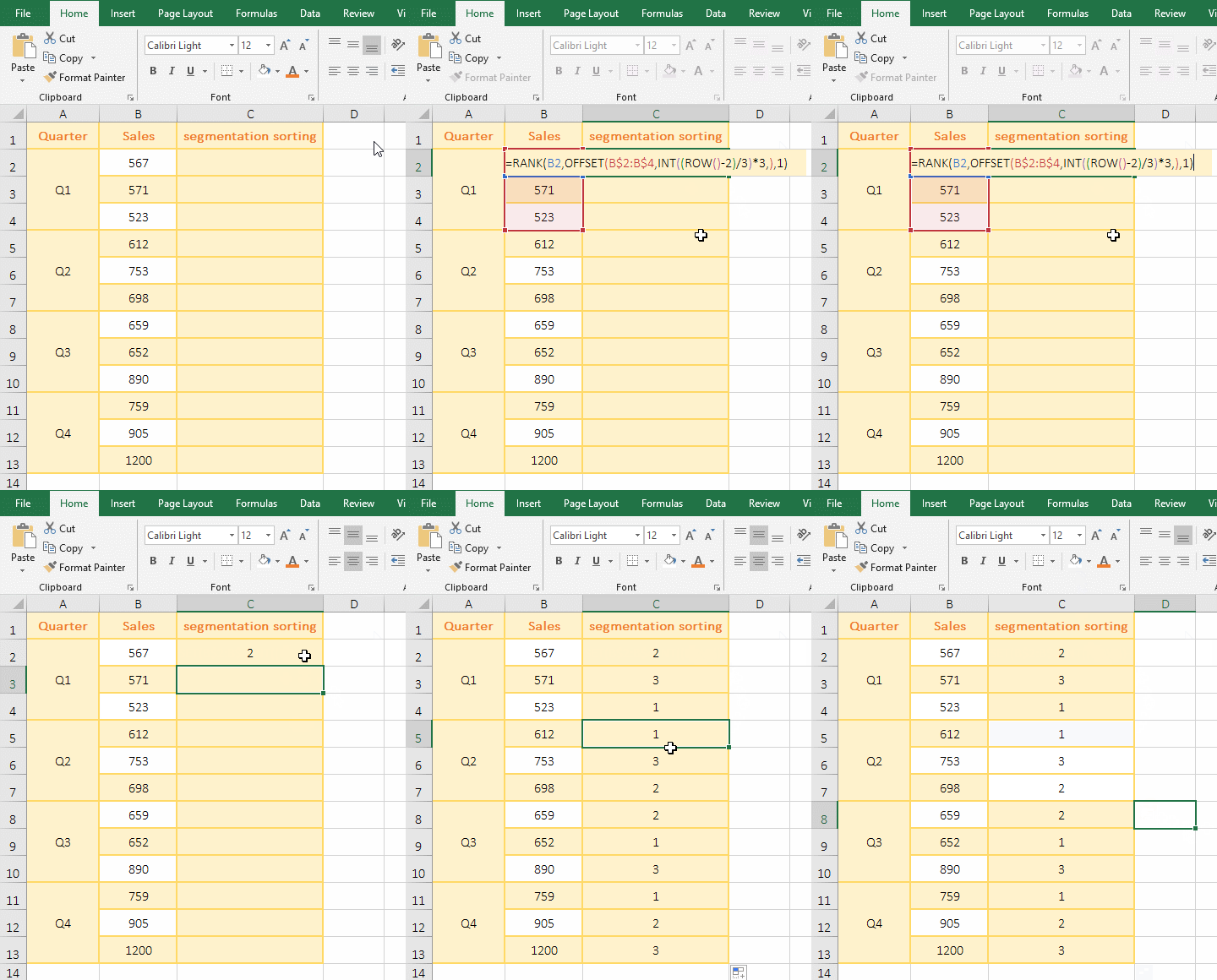
Figure 7

2. Formula =RANK(B2,OFFSET(B$2:B$4,INT((ROW()-2)/3)*3,),1) explanation:

A. 3 in the formula means 3 digits per section; ROW() is used to return the Row_Num of the row where the formula is located; Int function is used to round; INT((ROW()-2)/3)*3,) is used to calculate the number of rows which the OffSet function to move down.

B. B$2:B$4 is the first section; OFFSET(B$2:B$4,INT((ROW()-2)/3)*3,) is used to move to the next section, how is it implemented to move to the next section?

First section(B$2:B$4):

When the formula is in C2, ROW() returns 2, INT((ROW()-2)/3)*3 becomes INT((2-2)/3)*3, and the result is 0; then OFFSET(B$2 :B$4,INT((ROW()-2)/3)*3,) becomes OFFSET(B$2:B$4,0,), which means that B$2:B$4 is shifted down by 0 row, that is, no less Shift, then OFFSET(B$2:B$4,0,) returns B$2:B$4; then the formula becomes =RANK(B2,B$2:B$4), and finally returns the rank 2 of the number in B2 in B2 to B4.

When the formula is in C3, ROW() returns 3, (ROW()-2)/3 becomes INT(1/3), and then rounds up, the result is 0, the result of 0 * 3 is also 0; OffSet becomes OFFSET(B$2:B$4,0,); then the formula becomes =RANK(B3,B$2:B$4), and finally returns the rank 3 of the number in B3 in B2 to B4.

When the formula is in C4, ROW() returns 4, (ROW()-2)/3 becomes INT(2/3), and then rounds up, the result is 0, the result of 0 * 3 is also 0; OffSet becomes OFFSET(B$2:B$4,0,); then the formula becomes =RANK(B4,B$2:B$4), and finally returns the rank 1 of the number in B4 in B2 to B4.

Second section(B$5:B$7):

When the formula is in C5, ROW() returns 5, (ROW()-2)/3 becomes INT(3/3), and then rounds up, the result is 1, the result of 1 * 3 is also 3; OffSet becomes OFFSET(B$2:B$4,3,) means to shift B$2:B$4 down three rows, then B$2:B$4 becomes B$5:B$7, and it moves to the second section; then the formula becomes =RANK(B5,B$5:B$7), and finally returns the rank of the number in B5 in B$5:B$7; other and so on.

The process of B$2:B$4 is shifted down three rows by OFFSET(B$2:B$4,3,): Take B2 from B2:B4 for the first time, then return to the reference to cells rows 3 under B2, return B5; take B3 from B2:B4 for the second time, and then return the reference to cells rows 3 under B6, that is, return to B6; returns also the reference to B7 for the third time, thus the B$2:B$4 is moved down three rows.

(II) Rank + OffSet + Column combination to change the list of numbers into the row

1. If you want to change the numbers that have been ranked in column A into the row. Double-click cell C2, copy the formula =RANK(OFFA($A1,COLUMN()-3,),$A1:$A6) to C2, press Enter, return to 6. Select C2, move the mouse to the cell fill handle in the lower right corner of C2, after the mouse becomes the bold black plus, hold down the left button and drag to the right, dragging all the numbers until the end; the operation steps are as shown in Figure 8:

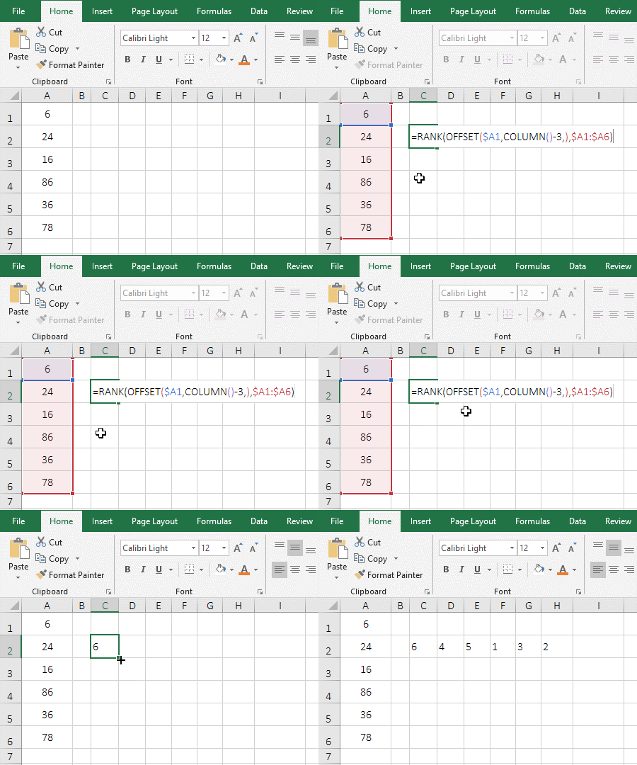
Figure 8

2. Formula =RANK(OFFSET($A1,COLUMN()-3,),$A1:$A6) explanation:

A. $A1 represents an absolute reference to the column, when dragged to the right, A1 will not become B1, C1, etc.; COLUMN() is used to return the Column_Num of the column that contains the formula.

B. OFFSET($A1,COLUMN()-3,) is used to return the values in A1 to A6, details as follows:

When the formula is in C2, COLUMN() returns 3, then OffSet becomes OFFSET($A1,3-3,), which means returning a reference to cell row 0 under A1, that is, returning a reference to A1, that is, returning 6; the formula becomes =RANK(6,$A1:$A6), and then the Rank function is used to return the rank 6 of 6 in A1:A6.

When the formula is in D2, COLUMN() returns 4, then OffSet becomes OFFSET($A1,4-3,), which means returning a reference to cell row 1 under A1, that is, returning a reference to A2, that is, returning 24; the formula becomes =RANK(24,$A1:$A6), then the Rank function is used to return the rank 4 of 24 in A1:A6; the others and so on.

VI, Excel rank without skipping numbers

If you want to rank the duplicate numbers side by side, and the rank don't skip numbers, for example, 5, 3, 3, 2, if you rank in descending order, ask both 3 to rank 2nd, and 2 Ranked third; which cannot be achieved with the Rank function, but can be achieved with other combinations of functions, as follows:

(I) Sum + If + CountIf

1. Also take the example which "Price" column are automatically ranked in descending and ascending order. Double-click cell E2, copy the formula =SUM(IF(C$2:C$7>=C2,1/COUNTIF(C$2:C$7,C$2:C$7),"")) to E2, press Ctrl + Shift + Enter, return 4; select E2, double-click the cell fill handle in the lower right corner of E2 to rank the remaining number; then double-click F2, copy the formula =SUM(IF(C$2:C$7<=C2,1/COUNTIF(C$2:C$7,C$2:C$7),"")) to F2, press Ctrl + Shift + Enter, return to 2, return the remaining position by double-clicking the cell fill handle; the operation steps are as shown in Figure 9:

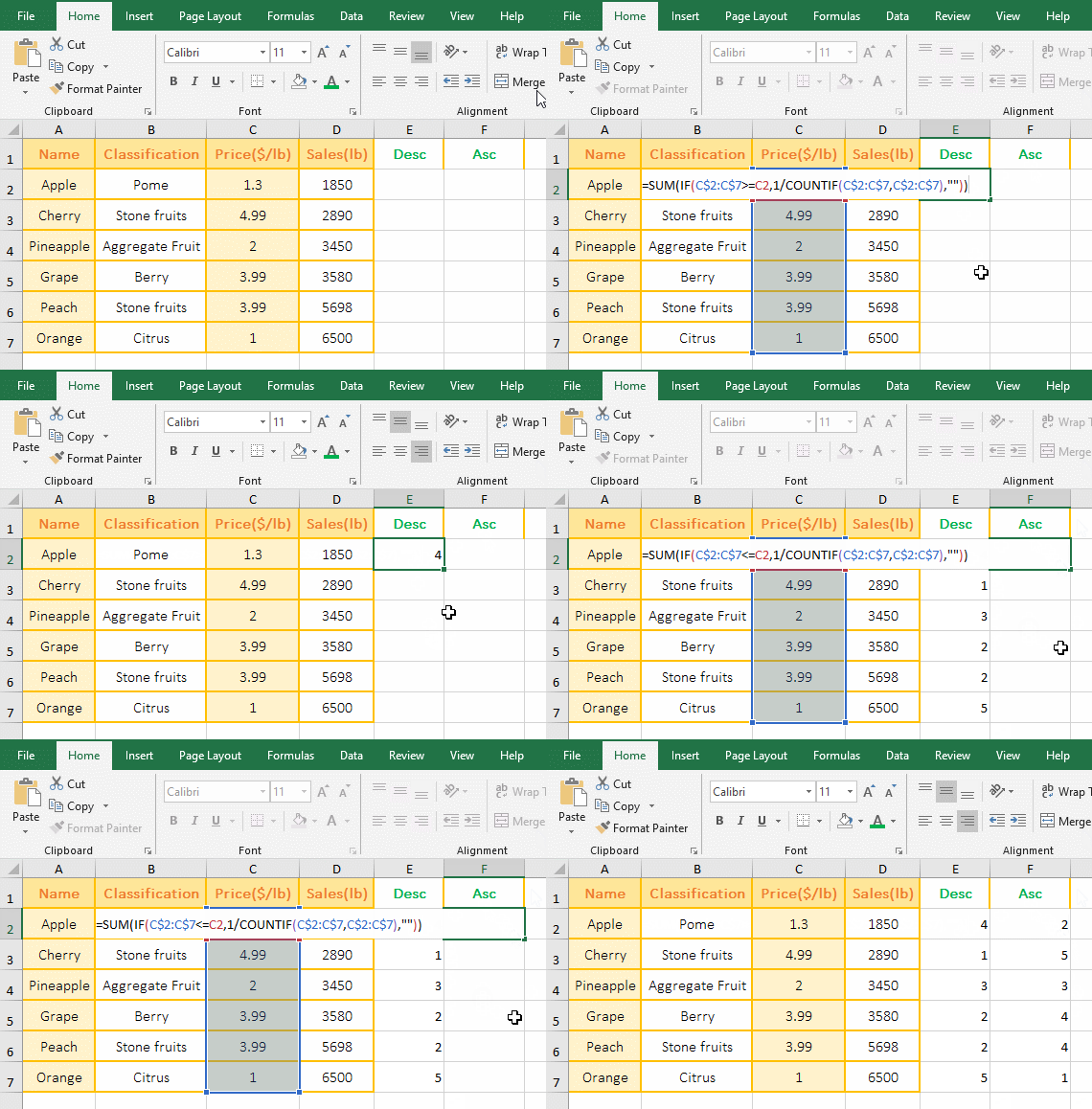
Figure 9

2. Descending order formula =SUM(IF(C$2:C$7>=C2,1/COUNTIF(C$2:C$7,C$2:C$7),"")) description:

A. The two key points which duplicate numbers are ranked without skipping numbers: One is to find the duplicate numbers, and the other is to increase the ranking after the duplicate number by one.

B. C$2:C$7 returns the value in C2 to C7 as an array. $ is an absolute reference to the row. When it is dragged down, C2 will not change to C3, C4, etc., C7 will not change to C8, C9, etc. To ensure that the number of C2:C7 is always taken.

C. 1/COUNTIF(C$2:C$7,C$2:C$7) is used to find duplicate numbers; C2(ie 1.3) is taken from C2:C7 on the first execution, then the number of C2 is counted in C2:C7, the result is 2; C3(ie 4.99) is taken from C2:C7 on the second execution, then the number of C3 is counted in C2:C7, the result is 1; the others and so on, and finally returns {1;1;1;2;2;1}.

D. Then 1/COUNTIF (C$2:C$7, C$2:C$7) becomes 1/{1;1;1;2;2;1}, further calculation, divide 1 by each element in the array, the result is {1;1;1;0.5;0.5;1}, so that the duplicate numbers(two 3.99) is changed to one, and the following steps will add two 0.5, which is actually filtering the duplicate numbers. It has already been introduced in the previous chapter.

E. C$2:C$7>=C2 is the criteria of If, used to find all the values in C2:C7 that are greater than or equal to C2; when executed, C2(ie 1.3) is taken for the first time, C2 >= C2 is established, return True; C3(ie 4.99) is taken out for the second time, C3 >= C2 is also established, and returns True; the others and so on, and finally returns {TRUE;TRUE;TRUE;TRUE;TRUE;FALSE}.

F. Then the formula becomes =SUM(IF({TRUE;TRUE;TRUE;TRUE;TRUE;FALSE},{1;1;1;0.5;0.5;1},"")), when executed, the first element True is taken from the conditional array for the first time. Since it is true, the element corresponding to the conditional array in the second array is returned, that is, the first element 1 of the second array is returned; the second element True is taken from the conditional array for the second time, because it is also True, the second element 1 of the second array is returned; the sixth element False is taken from the conditional array for the sixth time, because it is false, the third argument of if is returned; and so on, and finally return {1;1;1;0.5;0.5;""}.

G. The formula becomes =SUM({1;1;1;0.5;0.5;""}), and finally each element in the array is added by Sum, and only the numbers are added because the null value is ignored, so the result is 4; two 0.5 are the values of 3.99 in the duplicate numbers C5 and C6, 1 is a value greater than or equal to 1.3(ie 1.3 in C2), adding them exactly to the rank of the duplicate number 3.99.

In addition, this formula = SUM(IF(C$2:C$7<=C2,"",1/COUNTIF(C$2:C$7,C$2:C$7)))+1 can also achieve descending ranking, ie >= Change to <=, and the next two arguments of If are to be reversed, and 1 is added after the formula.

3. Ascending ranking formula =SUM(IF(C$2:C$7<=C2,1/COUNTIF(C$2:C$7,C$2:C$7),"")) description:

The difference between the ascending ranking formula and descending ranking formula is that the >= in the If criteria becomes <=, that is, finding all the numbers greater than or equal to the current cell(C2) becomes finding all the numbers less than or equal to the current cell.

(II) SumProduct + CountIf

1. Also take the example above. Double-click cell E2, copy the formula =SUMPRODUCT((C$2:C$7>=C2)/COUNTIF(C$2:C$7,C$2:C$7)) to E2, press Enter, return 4; select E2, return the ranking of the remaining numbers by double-clicking the cell fill handle; double-click F2, copy the formula =SUMPRODUCT((C$2:C$7<=C2)/COUNTIF(C$2:C$7,C$2:C$7)) to F2, press Enter, return to 2, and then double-click the cell fill handle to return the remaining ranking; the operation steps, as shown in Figure 10:

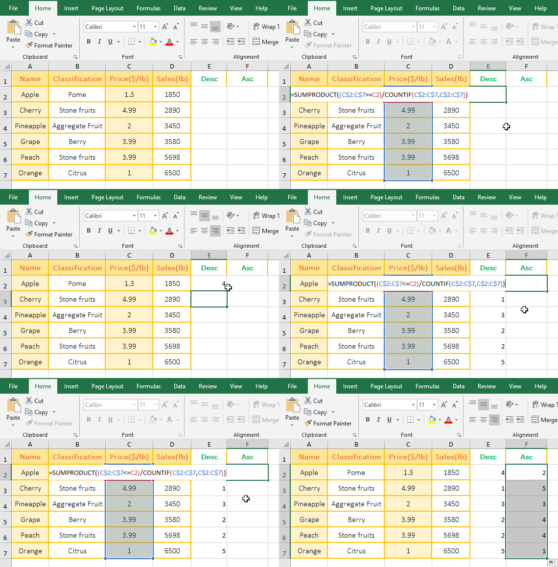
Figure 10

2. Descending ranking formula =SUMPRODUCT((C$2:C$7>=C2)/COUNTIF(C$2:C$7,C$2:C$7)) description:

A. Formula and Sum + If + CountIf is a meaning, but here SumProduct is used instead of Sum + If.

B. COUNTIF(C$2:C$7,C$2:C$7) returns {1;1;1;2;2;1};(C$2:C$7>=C2) returns {TRUE;TRUE;TRUE;TRUE;TRUE;FALSE}.

C. The formula becomes =SUMPRODUCT({TRUE;TRUE;TRUE;TRUE;TRUE;FALSE}/{1;1;1;2;2;1}), further calculation, take out the first elements TRUE and 1 from the numerator and denominator arrays for the first time, when calculated, TRUE is converted to 1, FALSE is converted to 0, 1/1 = 1; take the sixth elements FALSE and 1 from the numerator and denominator arrays for the sixth time ,0/1 = 0, Others and so on.

D. The formula becomes =SUMPRODUCT({1;1;1;0.5;0.5;0}), and the elements in the array are summed finally, and the result is 4, that is, the duplicate number 3.99 is ranked 4.

In addition, this formula =SUMPRODUCT((C$2:C$7>C2)*(1/COUNTIF(C$2:C$7,C$2:C$7)))+1 can also achieve descending ranking, that is, the critera C$2:C$7>C2 is extracted as an independent criteria, then 1/COUNTIF(C$2:C$7,C$2:C$7) is as the second criteria, and * is used to connect the two criteria to indicate "And" relationship, and finally add 1 to the formula.

3. Ascending ranking formula =SUMPRODUCT((C$2:C$7<=C2)/COUNTIF(C$2:C$7,C$2:C$7)) description:

The difference between the ascending ranking formula and the descending ranking formula is simply to change the >= in the numerator C$2:C$7<=C2 to <= to <=, that is, to find all the numbers greater than or equal to the current cell(C2) is changed to find all the numbers less than or equal to the current cell.

(III) Sum + If + FreQuency

1. Also take the example above. Double-click cell E2, copy the formula =SUM(--(IF(FREQUENCY(C$2:C$7,C$2:C$7),C$2:C$7>C2)))+1 to E2, press Ctrl + Shift + Enter, return 4; select E2, double-click the cell fill handle of E2 to return the ranking of the remaining numbers; then double-click F2, copy the formula =SUM(--(IF(FREQUENCY(C$2:C$7,C$2:C$7),C$2:C$7<=C2))) to F2, press Enter, return to 2, then double-click the cell fill handle of F2 to return the remaining ranking; the operation steps are as shown in Figure 11:

Figure 11

2. Descending ranking formula =SUM(--(IF(FREQUENCY(C$2:C$7,C$2:C$7),C$2:C$7>C2)))+1 description:

A. FREQUENCY(C$2:C$7,C$2:C$7) is used to find out the frequency of each number appears in the C2:C7. The function is a bit like COUNTIF(C$2:C$7, C$2:C$7)), but FreQuency counts only once for duplicate numbers, and CountIf counts twice.

When executing, 

First, take C2(ie 1.3) from the second argument, then count the number of values less than or equal to 1.3 and greater than 1 in C2:C7 (result is ), because C2:C7 is directly used the Bins_Array argument of the Frequency function (that is, the interval argument is divided into the values to be counted), and the value smaller than 1.3 is 1, so 1 and 1.3 are one interval.

Second, C3(ie 4.99) is taken from the second argument; similarly, the number of values(the result is 1) less than or equal to 4.99 and greater than 3.99 is counted in C2:C7.

Fourth, C5(3.99) is taken out from the second argument, and the number of values(the result is 2) less than or equal to 3.99 and greater than 2 is counted in C2:C7.

Fifth, C6(3.99) is taken out from the second argument, since C6 has been counted and no longer counted, the result is 0.

The others and so on, finally the array {1;1;1;2;0;1;0} is returned.

There are only 6 numbers in C2:C7, and why the returned array has 7 elements, because the array returned by the FreQuency function will have one more element than the Bins_Array parameter.

B. C$2:C$7>C2 returns {FALSE;TRUE;TRUE;TRUE;TRUE;FALSE}.

C. IF(FREQUENCY(C$2:C$7,C$2:C$7),C$2:C$7>C2) becomes IF({1;1;1;2;0;1;0},{FALSE;TRUE;TRUE;TRUE;TRUE;FALSE}); When executed, 

First, the first element 1 is taken from the conditional array, since it is regarded as true when the number greater than 0, it is regarded as false when the number less than 0, so the second argument of If is returned, that is, the element FALSE corresponding to 1 in the second array.

Second, the second element 1 is taken from the conditional array, since it is true, returns the second element TRUE in the second array; 

Fifth, the fifth element 0 is taken from the conditional array, because it is false, it returns the fifth argument of If, because the fifth argument is omitted, it returns FALSE by default;

The other and so on, and finally returns {FALSE;TRUE;TRUE;TRUE;FALSE;FALSE;FALSE}.

D. The formula becomes =SUM(--{FALSE;TRUE;TRUE;TRUE;FALSE;FALSE;FALSE})+1, further calculation, convert all elements of the array into numeric values, then the formula becomes =SUM({ 0;1;1;1;0;0;0})+1, -- is used to convert text or logical values into values, equivalent to the Value function, and finally adds the elements in the array and 1, the result is 4.

3. Ascending ranking formula =SUM(--(IF(FREQUENCY(C$2:C$7,C$2:C$7),C$2:C$7<=C2))) description:

The difference between the ascending ranking formula and the descending ranking formula is only to change the > in C$2:C$7>C2 to <=, that is, to find all the numbers larger than the current cell(C2) is changed to find all the numbers smaller than or equal to the current cell(C2), and remove the last 1 in the formula.