Excel column function usage(7 examples, with 1:1/$1:$1 and returns the sum of odd or even columns)

The Column function is used to return the column number of a reference to a cell or a range of cells in Excel; it can either omit or specify  arguments, if omitted, return the column number of the cell in which the formula is located; if you want to return the column number of the cell range to be referenced as an array, you need to press Ctrl + Shift + Enter. The Columns function is used to return the number of columns of an array or a range of cells to be referenced, it cannot omit arguments.

The Columns function is often used in combination with functions such as Index, Indirect, Char, SumProduct, Mod, If, Sum, and Row. For example, the Index + Column combination returns a reference to a cell specified by the row number and column number in the cell range to be referenced, Indirect + Char + Column + Row combination returns the content of the specified row and under it, and the SumProduct + Mod + Column combination adds even or odd columns.

I,  The syntax of Excel Column function and Columns function

1. Column function expression: COLUMN([Reference])

2. Columns function expression: COLUMNS(Array)

3. Description:

A. Column function is used to return the column number of the reference to a cell or a range. The argument Reference can be omitted, if omitted, the column number of the column in which the formula is located is returned. If Reference is a reference to a cell, the column number of that cell is returned. If Reference is a reference to a range of cells, if it is a horizontal reference(such as A1:C1), press Ctrl + Shift + Enter to return the column number of A1 to C1 as an array; press Enter to return only the column number of A1. Reference cannot reference multiple ranges.

B. Columns function is used to return the number of columns of the array or reference to a cell or a range, the argument Array can not be omitted.

II, The examples of Excel Column function

(I) Return the column number of the cell in which the formula is located or the specified cell

1. Select the cell B1, enter the formula =COLUMN(), press Enter, return 2; double-click A1, copy the formula =COLUMN(C1) to A1, press Enter, return to 3; the operation steps are as shown in Figure 1:

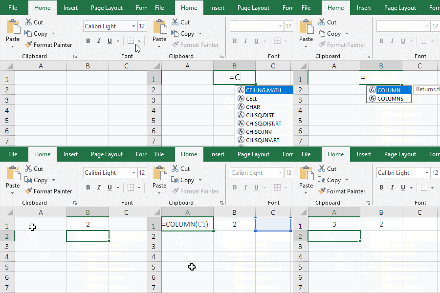
Figure 1

2. Description:

The formula =COLUMN() omits the argument, the column number of the cell in which the formula is located is returned by default; the formula is in B1, so the column number 2 of B1 is returned; the argument of formula =COLUMN(C1) is C1, although the formula is in cell A1, it still returns the number 3 of C1.

(II) Return the specified column number as an array

1. If you want to return the column numbers of A1 to D1 as an array. Double-click the cell E2, copy the formula =COLUMN(A1:D1) to E2, press Ctrl + Shift + Enter, return to 1, select E2, hold down the Alt key, press M and V respectively to open the "Evaluate Formula" window, press Enter to evaluate, the result is 1; double-click E3, copy the formula =INDEX(COLUMN(A1:D1),,2) to E3, press Ctrl + Shift + Enter, return 2, select E3, open the "Evaluate Formula" window with the same method, press Enter to evaluate, return an array of 1 to 4; the operation steps, as shown in Figure 2:

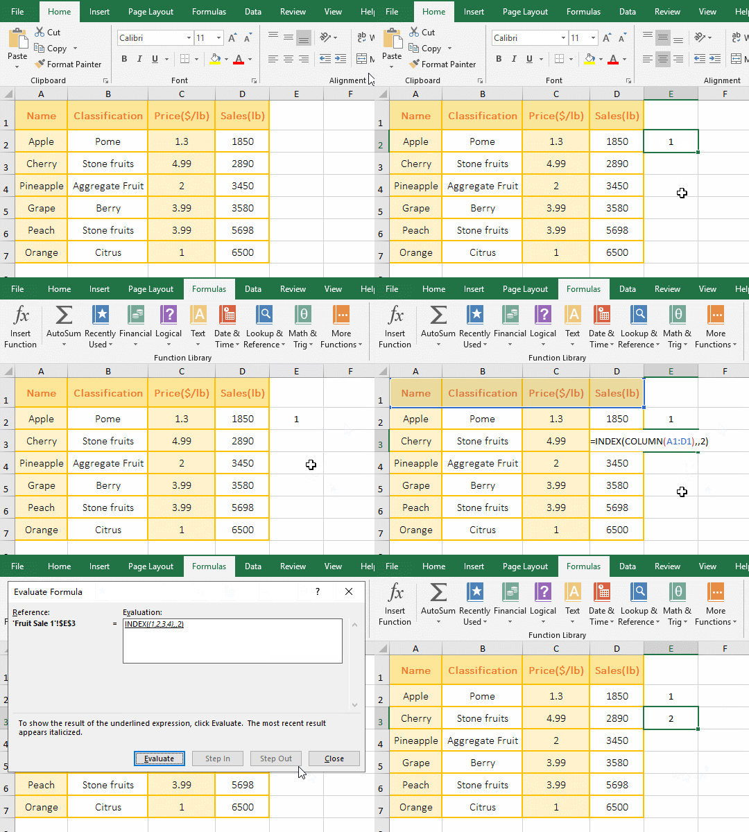
Figure 2

2. Formula description:

A. As you can see from the demo, although press Ctrl + Shift + Enter, the formula =COLUMN(A1:D1) still cannot return the array, because you need to put =COLUMN(A1:D1) in the referenced function to return the array. COLUMN(A1:D1) is inserted in the Index function and returns the array {1;2;3;4}.

B. The formula =INDEX(COLUMN(A1:D1),,2) is used to return the value or reference of value that are specified by the row number and column number in the array or range of cells to be referenced, COLUMN(A1:D1) which returns {1;2;3;4} is its first argument(ie array), the second argument is the rpw number(omitted), the third argument is the column number(value is 2); the meaning of the formula: returns the value of the second column in 1;2;3;4}, that is, returns 2.

(III) Return all column numbers Column(1:1) in row or column number Column(A:A) in column

1. Double-click the cell A2, copy the formula =INDEX(COLUMN( to A2, click row number 1 of the first row, automatically enter 1:1, then enter "), 3)", press Ctrl + Shift + Enter, return 3; double-click B2, copy =INDEX(COLUMN( to B2, click column number A of the first column, automatically enter A:A, then enter "),1)", press Ctrl + Shift + Enter, return 1; operation process steps, as shown in Figure 3:

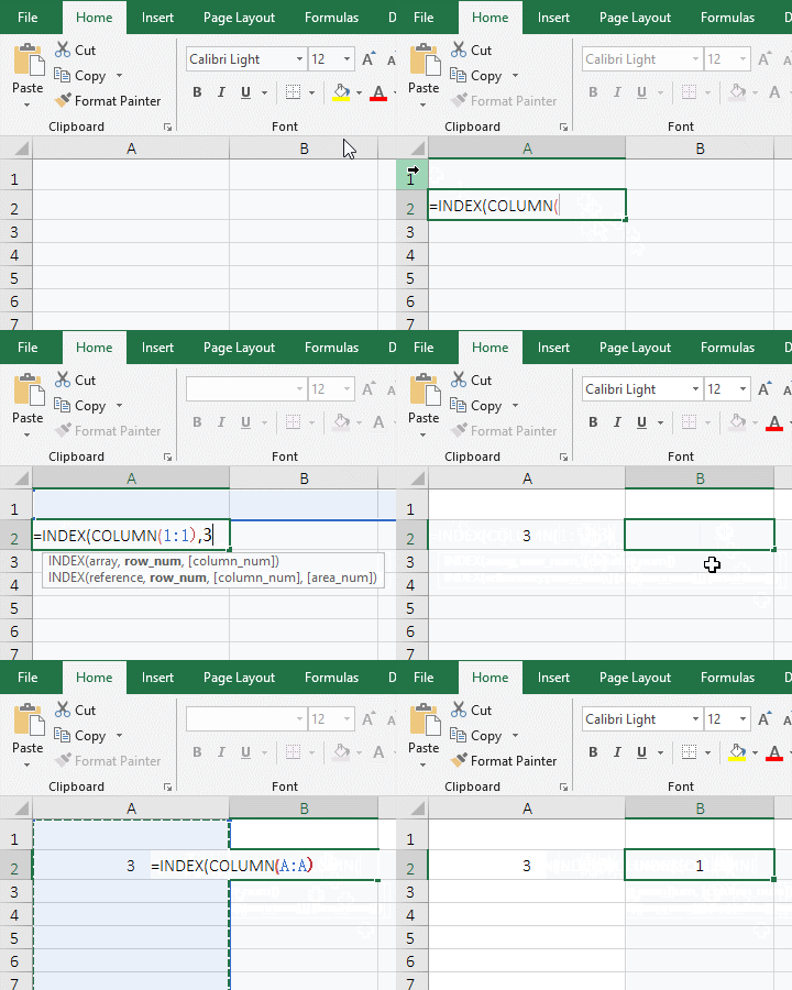
Figure 3

2. Formula description:

A. COLUMN(1:1) is used to return the column numbers of the first row as an array in the formula =INDEX(COLUMN(1:1),3), it is instead of COLUMN($1:$1), $ for absolute reference.

B. COLUMN(A:A) is used to return the column number of the first column as an array in the formula =INDEX(COLUMN(A:A),1), A:A means to refer to the first column, you can also instead of it with COLUMN($A:$A).

III, The examples of Excel Columns function

(I) Return the numbers of array

1. Double-click the cell A1, copy the formula =COLUMNS({3,8,4,7,9,2}) to A1, press Enter, return to 6 columns; double-click A1 again, change the second and fourth comma(,) to a semicolon(;) in the formula, press Enter, return 2 columns; the operation steps, as shown in Figure 4:

Figure 4

2. Formula description:

The formula =COLUMNS({3,8,4,7,9,2}) is used to return the number of columns in the array; the array has only one row with 6 elements, so returns 6 columns; and  the array of formula =COLUMNS({3,8;4,7;9,2}) has three rows, two elements per row, so two columns are returned; the semicolon(;) is the separator of row and row, and the comma(,) is the separation of the element from the element.

(II) Return the column number of the reference to a range of cells

Double-click the cell C3, copy the formula =COLUMNS(A1:D1) to C3, press Enter to return to 4; the operation steps are as shown in Figure 5:

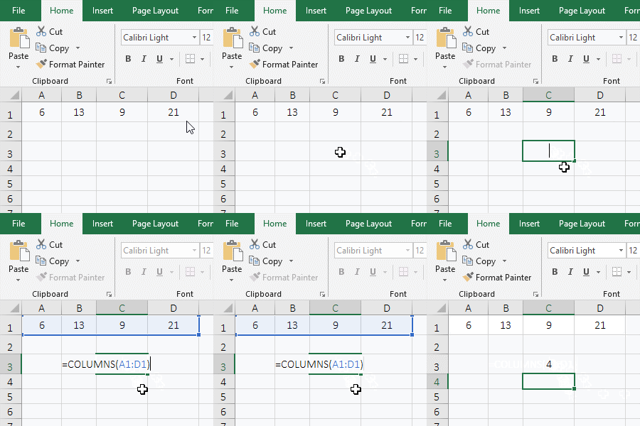
Figure 5

2. Formula description:

The formula =COLUMNS(A1:D1) is used to return the numbers in A1:D1, A1 to D1 are four columns, so 4 is returned.

IV, The extended application examples of Excel Column function

(I) Indirect + Char + Column + Row combination returns the content of the specified row and under it

1. If you want to return to the content of the fifth row and under in the table. Double-click the cell A9, copy the formula =INDIRECT(CHAR(COLUMN()+64)&ROW(A5)) to A9, press Enter, return to "Grape", select A9, and move the mouse to the cell fill handle in the lower right corner of A9, after the mouse changes to the bolk black plus sign (+), hold down the left button and drag to the right to return the content of the 5th row; select D9, drag down in the same way, then return to the content of rows 6 and 7; the operation process steps, as shown in Figure 6:

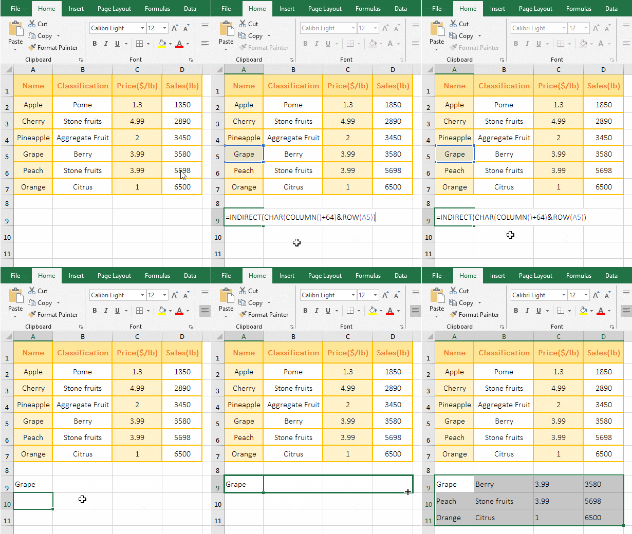
Figure 6

2. Formula =INDIRECT(CHAR(COLUMN()+64)&ROW(A5)) description:

A. COLUMN() is used to return the column number of the column in which the formula is located. When the formula is in A9, it returns 1; then CHAR(COLUMN()+64) becomes CHAR(1+64), 64 is the encoding of @ in ASCII code table, and 65 is the encoding of uppercase A. Char function is used to return the character corresponding to ASCII code, CHAR(65) returns A; COLUMN()+64 is used because COLUMN() returns B, C, D, etc. Column numbers 2, 3, 4 when dragging to the right, 64 + 2 are the ASCII encoding of B, 64 + 3 is the ASCII encoding of C, and so on, so that the column number of the cells that are passed when dragging right is returned, then return the letters of their corresponding columns with the Char function.

B. ROW(A5) is used to return the row number 5 of A5; when dragging down, A5 will change to A6, then ROW(A6) will return the row number 6 of A6; the others and so on.

C. The formula becomes =INDIRECT("A"&5), and finally returns a reference to A5 with the Indirect function, which returns the content "Grape" in A5.

(II) SumProduct + Mod + Column combination returns the sum of odd or even columns

1. Return the sum of the even columns; double-click the cell E11, copy the formula =SUMPRODUCT((MOD(COLUMN($B:$E),2)=COLUMN(A1))*B$2:E$9) to E11, press Enter, returns the summation result 1338.5. Return the sum of the odd columns; double-click E12, copy the formula =SUMPRODUCT((MOD(COLUMN($B:$E),2)=0)*B$2:E$9) to E12, press Enter, return to 1516.12. The process steps are shown in Figure 7:

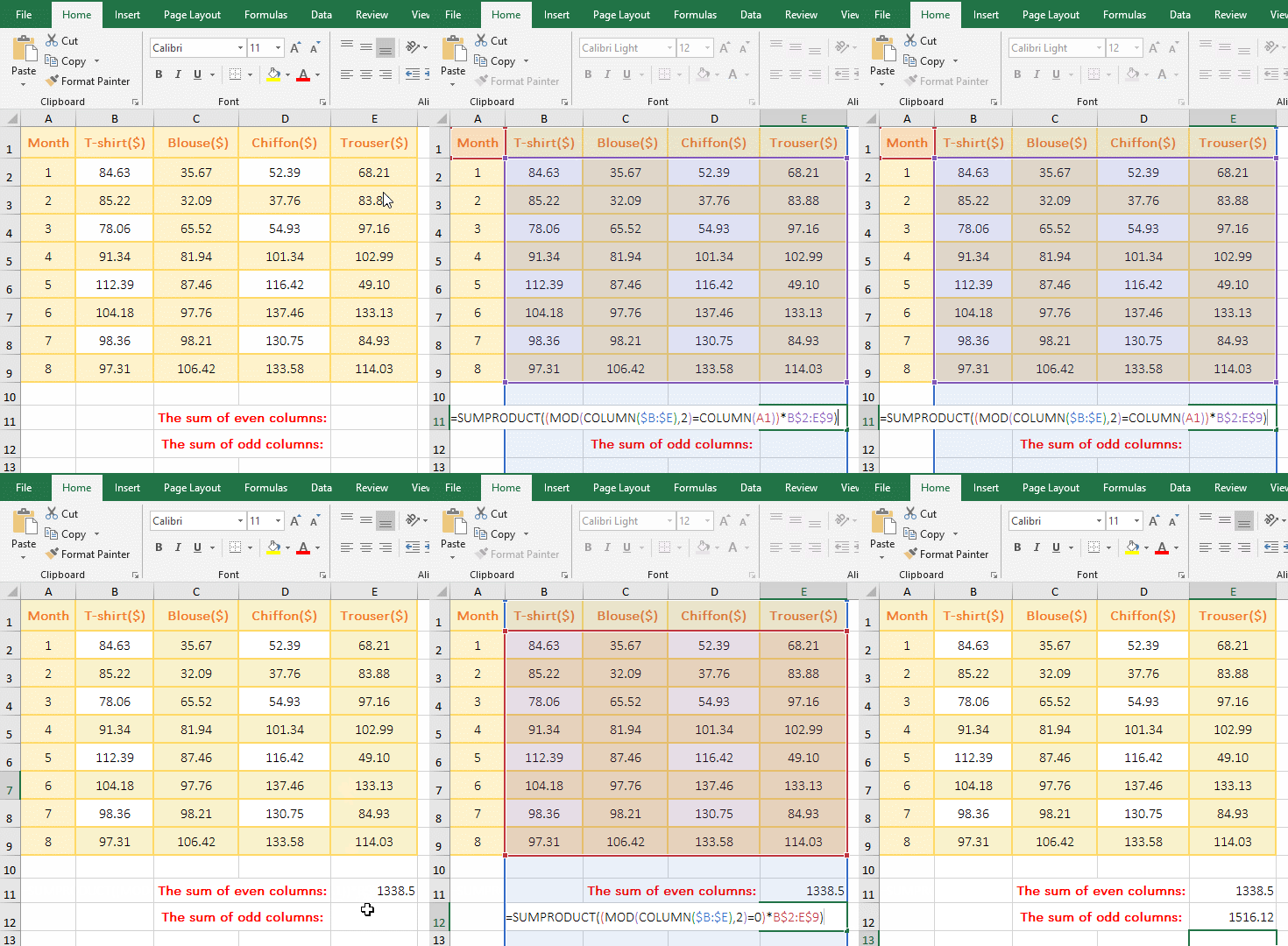
Figure 7

2. The formula of returning the sum of the even columns =SUMPRODUCT((MOD(COLUMN($B:$E),2)=COLUMN(A1))*B$2:E$9) explanation:

A. $B represents an absolute reference to column B, to ensure that the column B does not change column C, D, etc. when dragging right; $B:$E means always sum in column B to E; COLUMN($B:$E) returns the column number of B to E as an array, which returns {2;3;4;5}.

B. Then MOD(COLUMN($B:$ E),2) becomes MOD({2;3;4;5},2), and then each element in the array is modulo 2; first, 2 is taken out from the array, then it is modulo with 2(that is, take the remainder), the result is 0; second, 3 is taken from the array, then modulo with 2, the result is 1; the other and so on, and finally returns {0;1;0;1}. Modulo is used to find all even columns.

C. COLUMN(A1) is used to return the column number 1 of A1; then MOD(COLUMN($B:$E),2)=COLUMN(A1) becomes {0;1;0;1}={1}, further calculations, each element is taken from the array and compared with 1, if it is equal to 1, it returns True, otherwise it returns False, and finally returns {FALSE;TRUE;FALSE;TRUE}.

D. The formula becomes =SUMPRODUCT({FALSE;TRUE;FALSE;TRUE}*B$2:E$9), further calculation, first, the first element FALSE is taken from the array, and the B2 in B2:E9 corresponding it is returned, because it is false, it returns 0. 

Second, the second element TRUE is taken out from the array, and the C2 in B2:E9 corresponding it is returned, since it is true, it returns the value 35.67 in C2.

Third, The third element FALSE is taken from the array, and the D2 in B2:E9 corresponding it is returned, since it is false, it returns 0; 

The others and so on, and finally returns {0,35.67,0,68.21; 0,32.09,0,83.88; 0,65.52,0,97.16; 0,81.94,0,102.99; 0,87.46,0,49.1; 1,97.76,0,133.13; 0,98.21,0,84.93; 0,106.42,0,114.03}.

E. The formula is further changed to =SUMPRODUCT({0,35.67,0,68.21; 0,32.09,0,83.88; 0,65.52,0,97.16; 0,81.94,0,102.99; 0,87.46,0,49.1; 1,97.76,0,133.13; 0,98.21,0,84.93; 0,106.42,0,114.03}), and finally the elements in the array are summed, and the result is 1338.5.

Hint: Column B is the first column in $B:$E in the above formula. If the column A is the first column, it is the sum of the odd columns.

3. Return the sum of odd-numbered columns =SUMPRODUCT((MOD(COLUMN($B:$E),2)=0)*B$2:E$9) explanation:

The difference between the formula of returning the sum of odd-numbered columns and even-numbered columns is that the former finds the odd-numbered column with the modulo to be 0, and the latter uses the modulo to be 1 to find the even-numbered column, that is, the former uses MOD(COLUMN($B:$E) , 2) = 0 find the odd column, the latter find the even column with MOD(COLUMN($B:$ E),2)=COLUMN (A1)(Note: here is column B is the first column in $B:$E), everything else is the same.