Excel CountIf usage, include greater than or equal and multiple criteria examples

The CountIf function is used to count the number of cells in a specified range that satisfy a certain condition in excel; it has only two arguments, one is the statistical range, and the other is the criteria, the criteria cannot exceed 255 characters, if it is more than, use the Concatenate function or the concatenate operator &. The criteria are only *, ?, >, <, etc., and some special statistics can be completed. 

If the CountIf function needs to implement multi-condition statistics, it needs to be combined with If, OffSet, and Sum functions, and sometimes the condition needs to use an array. For example, the Sum + If + CountIf function combination realizes that the counted result do not contain empty and duplicate values. The Sum + CountIf + array condition implements statistics that satisfy both conditions within the same range.

I, Excel CountIf function syntax

1. Expression: COUNTIF(Range, Criteria)

2. Description:

A. Range can be an array or a reference to a cell or cells.

B. The Criteria can be a single number or text, or an expression or function; but the characters in Criteria can not exceed 255, otherwise it will return an error; if the Criteria exceeds 255 characters, you can split them into multiple long strings And then concatenate them with the Concatenate function or the concatenate operator &, for example: "long character 1..." & "long string 2...". In addition, the Criteria ignores the case of letters.

C. You can use the wildcard question mark(?) and the asterisk(*) in the Criteria. The question mark indicates any character, the asterisk indicates any one or a string of characters. If you want to find the question mark or asterisk, you need to add an escape character before them; such as: look up the question mark, the expression should be written like this ~?; look for the asterisk, the expression should be written like this ~*.

D. When counting the number of texts, you cannot include leading and trailing spaces, and you cannot have single and double quotes inconsistent and non-printing characters; otherwise, the CountIf function may return unpredictable values. When there are spaces before or after the statistical text, you can use the Trim function to remove them; when there are non-printing characters, you can use the Clean function to remove them.

II, The examples of Excel CountIf function

(I) Examples of Criteria for text and counts nulls

1. Double-click the cell D2, copy the formula =COUNTIF(C1:C10,"Manager") to D2, press Enter, return to the counted result 2; double-click D2 again, remove the "manager" in the double quotes, press Enter, return to 1; the operation process steps, as shown in Figure 1:

Figure 1

2. Formula description:

C1:C10 is the counted Range, and "Manager" is the Criteria in the =COUNTIF(C1:C10,"Manager"), meaning: the number of "Manager" is counted in C1 to C10; when the Criteria is "", the number of count null values, there is only one empty cell in C1:C10, so the counted result is 1.

(II) The Criteria is an expression

1. If you want to count the number of fruits sold greater than or equal to 1000. Double-click the cell D8, copy the formula =COUNTIF(D2:D7,">=1000") to D8, press Enter, return to the counted result 6; the operation steps, as shown in Figure 2:

Figure 2

2. The formula =COUNTIF(D2:D7,">=1000") has the Criteria ">=1000", which means: the number that is greater than or equal to 1000 is counted in D2:D7; in addition, ">=1000" You can also write ">"&"1000", that is, write the greater than and the number separately, and then connect them with the concatenate operator &.

(III) Examples of functions in the Criteria(Excel countif greater than formula)

1. If you want to count the number of fruits sold more than the average. Double-click the cell D8, copy the formula =COUNTIF(D2:D7,">"&AVERAGE(D2:D7)) to D8, press Enter, return to the statistical result 3; the operation steps are as shown in Figure 3:

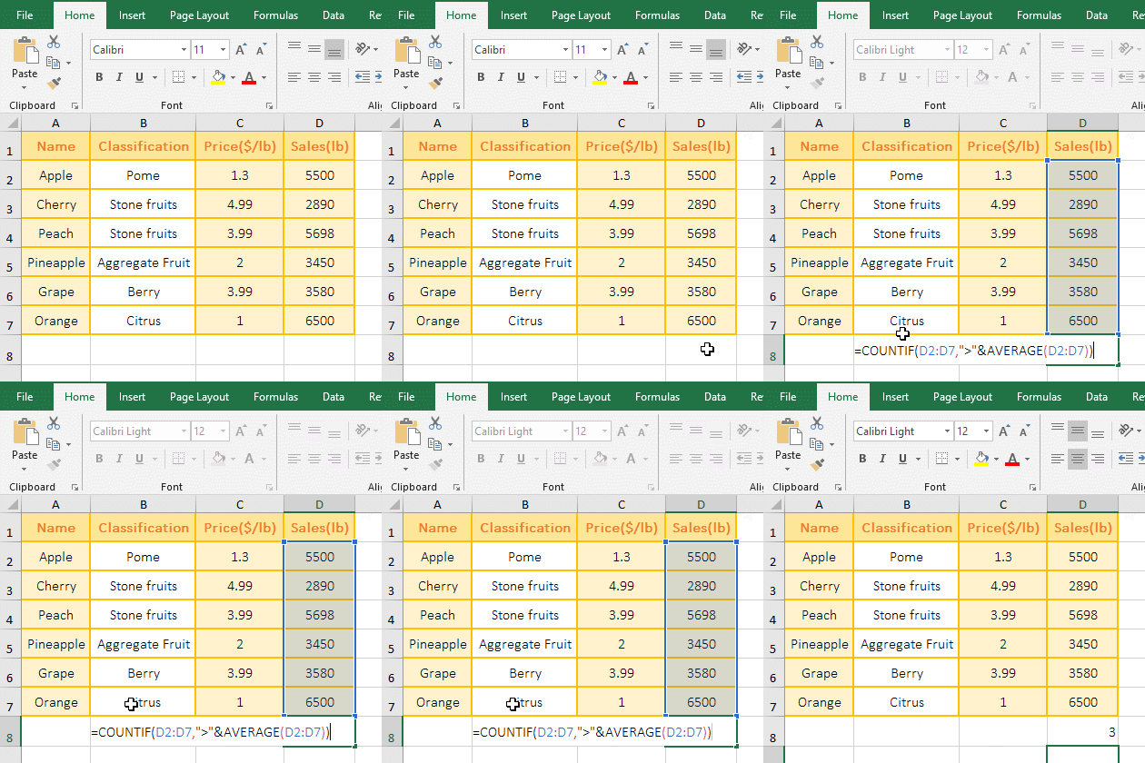
Figure 3

2.  The Criteria is ">"&AVERAGE (D2:D7) in the formula =COUNTIF(D2:D7,">"&AVERAGE(D2:D7)), the AVERAGE(D2:D7) in Criteria is used to calculate average in D2:D7(result is 4603), and then use & to connect the greater than and the number to form the Criteria, namely ">4603".

(IV) Examples of wildcards ? and * in the Criteria

1. If you want to count the number of employees begins with an S. Double-click the cell D2, copy the formula =COUNTIF(A2:A9,"S?????") to D2, press Enter, return to the counted result 1; double-click D2 again, change the ????? to * in the formula, press Enter, returns 2; the operation process steps, as shown in Figure 4:

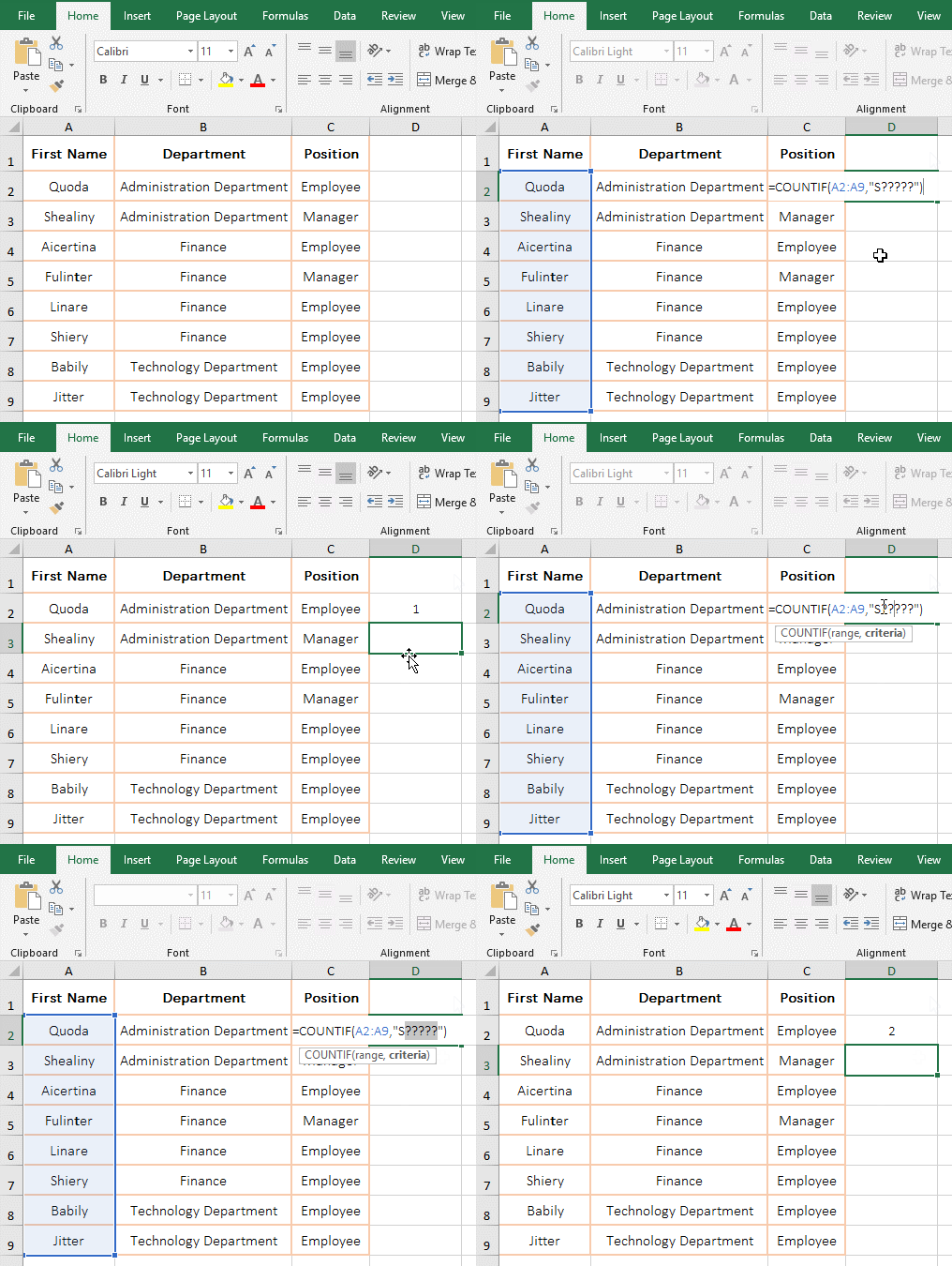
Figure 4

2. The formula =COUNTIF(A2:A9,"S?????") has the Criteria "S?????", which means "start with "S" and only two Characters after "
S"; when the Criteria is changed to "S*", it means "start with S", and there can be one or more arbitrary characters after "S". There are wildcards ? and * in the condition have been introduced many times in the previous chapter. If you want to know more ways to find, you can refer to the "How to use hlookup in excel(7 hlookup example, combine Match function)".

3. Examples of conditions * and ?*

A. The Criteria is *. Double-click the cell E9, copy the formula =COUNTIF(D1:D8,"*") to E9, press Enter, return to the counted result 2; double-click E8, remove the formula that returns empty (""), press Enter, and the counted result becomes 1; the text in E1 is deleted, and the counted result becomes 0. The demo is shown in Figure 5:

Figure 5

B. The Criteria is ?*. Double-click the cell E9, copy the formula =COUNTIF(D1:D8,"?*") to E9, press Enter, return to the counted result 1; double-click E8, change "" to "", and the counted result will be 2; Delete the text in E1, the counted result becomes 1, the demo is shown in Figure 6:

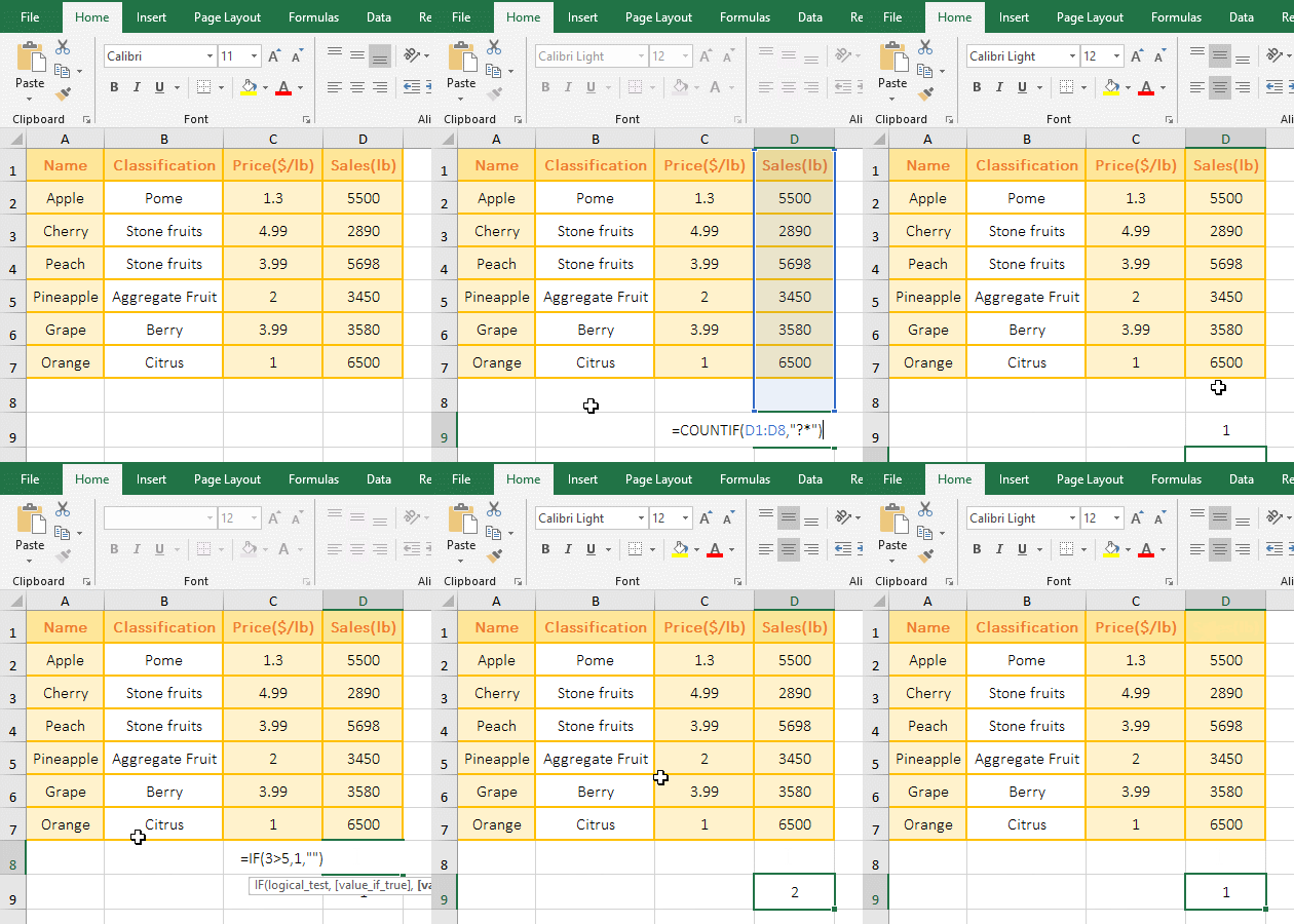
Figure 6

The difference between * and ?*: * can be one or more characters(including null ""), ?* must have at least two characters or a null value "", the two problems have been explained in the demo.

(V) Several special examples

1. Double-click the cell B11, copy the formula =COUNTIF(B2:B11,">=!") to B12, press Enter, return to the counted result 8; double-click B11, it is an empty cell, then double-click B10, there is a formula inside, double-click B7, press space to add a space before the "Finance", press Enter, the counted result becomes 7.

Copy the formula =COUNTIF(B2:B11,"><") to B13, press Enter, return the counted result 7, double-click B7, delete the space before the "Finance", the counted results in B11 and B12 become 8.

Double-click B14, copy the formula =COUNTIF(B2:B11,">""") to B14, press Enter, return to the counted result 8, double-click B7, add a space before the "Finance", the statistical results of B11, B12 and B13 become 7.

Double-click C12, copy the formula =COUNTIF(B2:B11,"<>") to C12, press Enter, return to the counted result 9; the operation process steps, as shown in Figure 7:

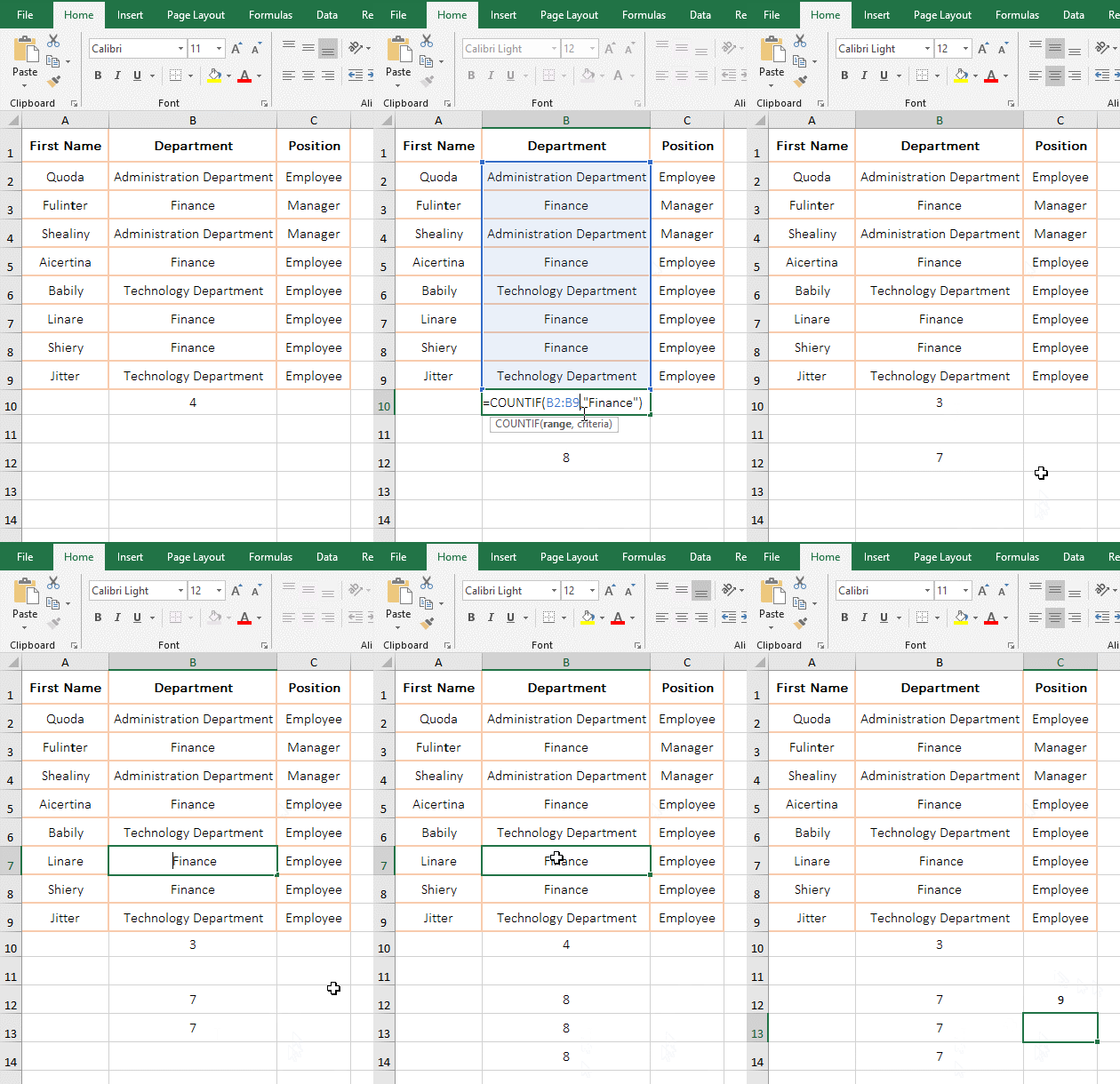
Figure 7

2. Formula description:

The formula =COUNTIF(B2:B11,">=!"), =COUNTIF(B2:B11,"><") and =COUNTIF(B2:B11,">""") have the same counted results, they do not contain Cells with formulas, empty cell, and cell with space before the text; and formula =COUNTIF(B2:B10,"<>") contains cell with formulas and do not contain empty cell.

III, Excel CountIf function extension use case

(I) The Sum + If + CountIf function combination realizes that the statistics are not empty and do not contain duplicate values.

1. Double-click the cell B10, copy the formula =SUM(IF(B2:B9<>"",1/COUNTIF(B2:B9,B2:B9))) to B10, press Ctrl + Shift + Enter to return to statistics result 3, the operation process steps, as shown in Figure 8:

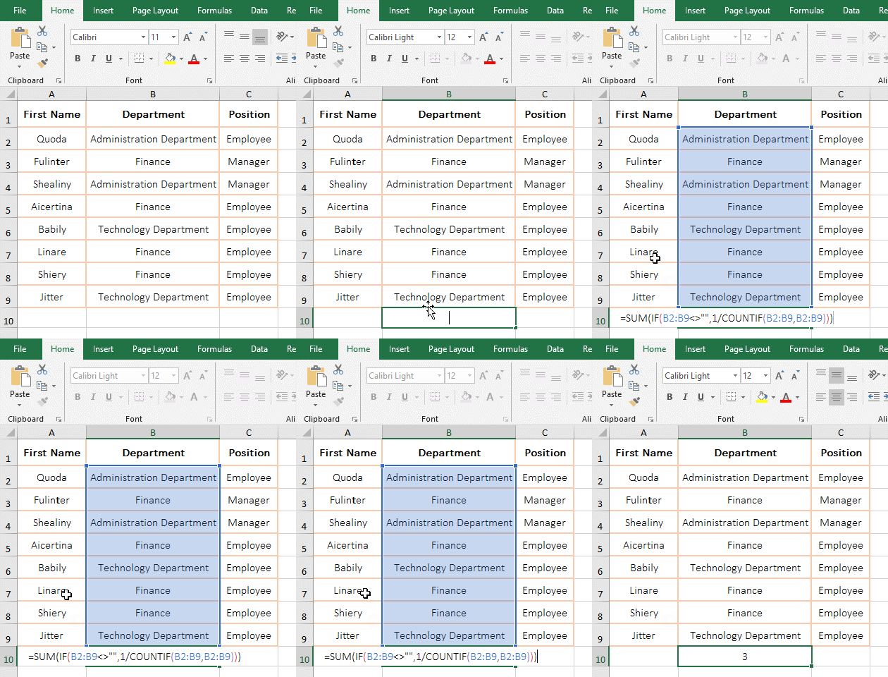
Figure 8

2. The formula =SUM(IF(B2:B9<>"",1/COUNTIF(B2:B9,B2:B9))) description:

A. B2:B9 is used to return all values in B2 to B9 as an array, namely {"Administration Department"; "Finance"; "Administration Department"; "Finance"; "Technology Department"; "Finance" ; "Finance";"Technology Department"}.

B. When COUNTIF(B2:B9,B2:B9) is executed, take B2(ie "Administration Department") from B2:B9 for the first time, then count the number of B2 in B2:B9, the result is 2; count the number of B3 in B2:B8 for the second time, the result is 4; the others and so on, and finally return {2;4;2;4;2;4;4;2}.

C. 1/COUNTIF(B2:B9,B2:B9) becomes 1/COUNTIF({2;4;2;4;2;4;4;2}), then divide 1 by each element in the array, the result returns {0.5;0.25;0.5;0.25; 0.5;0.25;0.25;0.5}; the effect of this step is to treat the total number of repeated values as 1, for example, repeating 2, each 1/2 is equal to 0.5, further calculation and then two 0.5 Add up, it happens to be 1, that is, remove a duplicate.

D. B2:B9<>"" means: each time an element is taken from B2:B9, if it is not empty, it returns True, otherwise it returns False; finally it returns {TRUE;TRUE;TRUE;TRUE;TRUE;TRUE;TRUE;TRUE}.

E. Then the formula becomes =SUM(IF({TRUE;TRUE;TRUE;TRUE;TRUE;TRUE;TRUE;TRUE},{0.5;0.25;0.5;0.25; 0.5;0.25;0.25;0.5})), followed by The first element TRUE is taken from the Criteria array of If. Since it is true, the corresponding element in the second array is returned, it is 0.5; until each element of the Critieria array are taken, and finally returns {0.5;0.25;0.5;0.25; 0.5;0.25;0.25;0.5}; then the formula becomes =SUM({0.5;0.25;0.5;0.25; 0.5;0.25;0.25;0.5}), and adds each element in the array finally, the result is 3.

(II) OffSet + CountIf function combination to achieve segmentation statistics

OffSet + CountIf to achieve segmentation statistics, please see the "How to use offset function in excel, include it and Sum, Match, CountIf combination in formula".

(III) Excel Countif multiple criteria

1. If you want to count the number of salespeople with Total sales of 50,000 to 80,000. Double-click the cell C10, copy the formula =SUM(COUNTIF(C2:C9,{">=50000",">80000"})*{1,-1}) to C10, press Enter to return to the statistical result 3. Operation process steps, as shown in Figure 9:

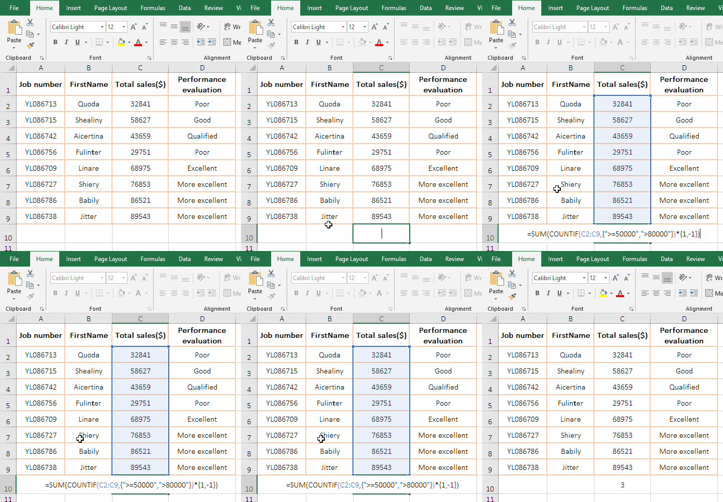
Figure 9

2. Formula =SUM(COUNTIF(C2:C9,{">=50000",">80000"})*{1,-1}) explanation(Excel countif greater than formula):

A. C2:C9 is the counted range of CountIf function, {">=50000", ">80000"} is the Criteria, it is an array, there are two Criteria, the first one is ">=50000", the second is ">80000", which means: count the number of greater than or equal to 50000 in C2:C8 for the first time, the result is 5; then count the number greater than 80000, the result is 2.

B. The formula becomes =SUM({5,2}*{1,-1}), and then, the corresponding elements of the two arrays are multiplied, and the formula becomes =SUM({5,-2}), and finally adds each elements in array and the result is 3. The key to this method is to count all the numbers greater than or equal to 50,000 for first time, then count the number greater than 80,000, and then use the former to reduce the latter.

3. The formulas for counting other ranges are:

A. Greater than 50000 and less than 80000: =SUM(COUNTIF(C2:C9,{">50000",">=80000"})*{1,-1})

B. Greater than or equal to 50000 and less than 80000: =SUM(COUNTIF (C2:C9,{">=50000",">= 80000"})*{1,-1}) or =SUM(COUNTIF(C2:C9,">="&{50000,80000})*{1,-1})

C. Greater than 50000 and less than or equal to 80000: =SUM(COUNTIF(C2:C8,{">50000",">80000"})*{1,-1}) or =COUNTIF(C2:C8,">50000" )- COUNTIF(C2:C8,">80000")