How to subtract in excel(7 examples, include Subtraction with criteria in formula)

There are two ways to calculate subtraction in Excel, one is to use the addition function(that is, the summation function) Sum, and the other is to use the minus sign. When calculating the subtraction with the Sum function, you only need to add a minus sign before the subtraction; use the minus sign to calculate the number by one minus one.

If you encounter a conditional subtraction, you need to use the If function to determine the condition; if you encounter the digital with unit, you need to use the Left function and the Find function to intercept the number, and then calculate; if required that the number that is involved in the calculation must have the ID, and it needs to be implemented in conjunction with the Indirect + Match + Row function; if you want to reduce all the numbers in the table by one, you need to use the paste special; in the calculation of the subtraction process.

I, The description of subtract function in excel

Excel does not provide directly a subtraction function, the subtraction operation requires the addition function, that is, the summation function Sum, the difference is that you only need to add a minus sign (negative sign) before the number to be subtracted. In addition, you can also use the minus sign(ie -) for subtraction.

II, How to subtract in excel

(I) Subtract two numbers

1. If you want to subtract the number in column A from the number in column B. Double-click the cell C1, copy the formula =SUM(-A1,B1) to C1, press Enter, return to 201; select C1, move the mouse to the cell fill handle in the lower right corner of C1, and after the mouse turns the bold black plus sign, click the left button to return the result of remaining numbers; the operation steps are as shown in Figure 1:

Figure 1

2. Description:

The - before A1 means minus in the formula =SUM(-A1,B1), the meaning of the formula is: subtract A1 from B1, that is, use the Sum function to calculate the subtraction by adding a minus sign(negative sign) before the subtrahend.

(II) The result of the subtraction is negative and is converted to a positive number by the absolute value.

1. If you want to substract the number in column B from the number in column A, the number in column A is small, and the number in column B is large. Double-click B1, copy the formula =SUM(A1,-B1) to C1, press Enter, return to -201; double-click C1 to add the absolute value function ABS into the formula, then the formula becomes =ABS(SUM(A1,-B1)), press Enter, return to 201; operation steps, as shown in Figure 2:

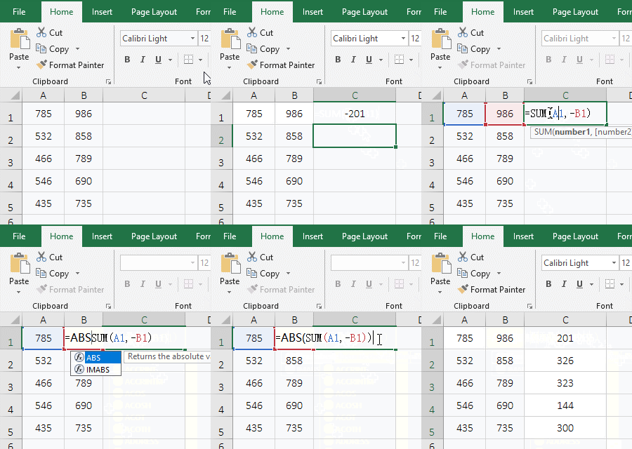
Figure 2

2. Formula description:

The formula =SUM(A1,-B1) returns a negative number, if a subtraction is required to return a positive number, just add the absolute value function ABS.

III, How to subtract in excel(with the minus sign)

1. Select the cell C1, enter the formula =B1-A1, press Enter, return to 201; select C2, enter the formula =A2-B2, press Enter, return to -326, double-click C2, and add the absolute value function ABS into the formula, the formula becomes =ABS(A2-B2), press Enter, return to 326; the operation steps, as shown in Figure 3:

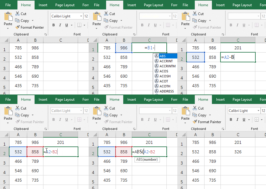
Figure 3

2. Formula description:

 Subtract one number from the other when calculating the subtraction with a minus sign. If the result is negative and you want to return a positive number, add the absolute value function ABS.

IV, The extended application examples of subtraction function in Excel

(I) Subtraction of digital with units

1. If you want to calculate the difference between January and February sales, and the sales volume in January with units. Double-click the cell C2, copy the formula =LEFT(A2,FIND("lb",A2)-1)-B2 to C2, press Enter, return to 247; select C2, and double-click the cell fill handle of C2 to return the remaining difference in sales; the operational steps, as shown in Figure 4:

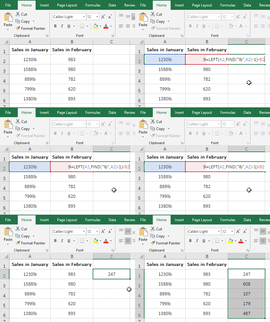
Figure 4

2. Formula =LEFT(A2,FIND("lb",A2)-1)-B2 explanation:

A. FIND("lb",A2) is used to find the position of "lb" in A2, the result is 4, then it is as the number of characters to extract numbers next. The reason why you need to use the Find function to return the number of digits to be extracted is because the number of digits are different in different cells in column A, and there are "lb" after the number, as long as the position of the "lb" is returned in the text and is reduced 1, you can accurately calculate the number of numbers.

B. Then =LEFT(A2,FIND("lb",A2)-1) becomes LEFT(A2,4-1), further calculation, intercept three characters from the left side of A2 with Left function, the result is 1230.

C. The formula becomes =1230-B2, B2 is 983, the two numbers are subtracted, and the result is 247.

(II) Subtraction with criteria

1. Requirement: If B2 is not empty, subtract B2 from A2; otherwise, if C2 is not empty, subtract C2 from A2; otherwise, if D2 is not empty, subtract D2 from A2; otherwise, return empty text. Double-click the cell E2, copy the formula =IF(B2<>"",A2-B2,IF(C2<>"",A2-C2,IF(D2<>"",A2-D2,""))) to E2, press Enter, return to 3; select E2, double-click E2's cell fill handle to return the result of the remaining values; the operation steps are as shown in Figure 5:

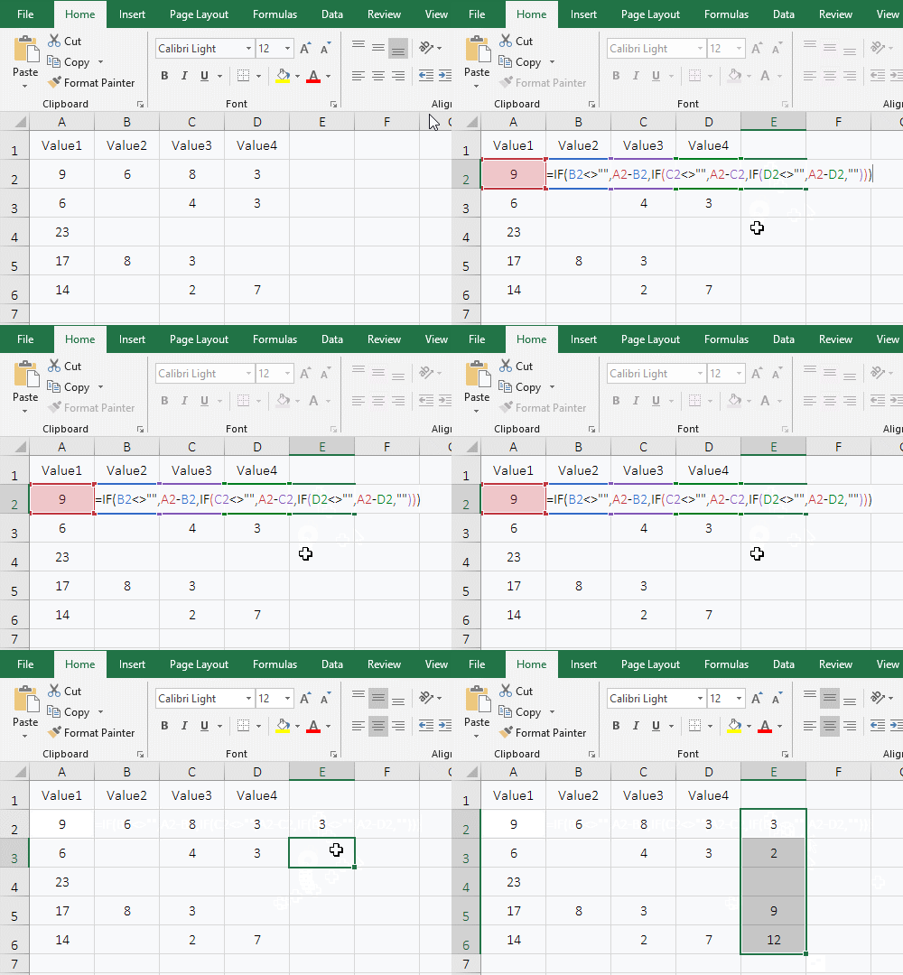
Figure 5

2. Formula =IF(B2<>"",A2-B2,IF(C2<>"",A2-C2,IF(D2<>"",A2-D2,""))) description:

A. The formula is nested with two If, starting from the outermost If; first, take the criteria B2<>"" of the outermost If, if it is established (that is, B2 is not empty), then execute A2-B2, otherwise execute IF(C2<>"",A2-C2,IF(D2<>"",A2-D2,"")); because B2 is 6 is not empty, so execute A2-B2, that is 9-6.

B. When the formula is in E3, the formula becomes =IF(B3<>"",A3-B3,IF(C3<>"",A3-C3,IF(D3<>"",A3-D3,""))), since B3 is empty, execute IF(C3<>"",A3-C3,IF(D3<>"",A3-D3,"")); C3 is 4, so C3<>" " established, execute A3-C3, ie 6-4.

C. When the formula is at E4, the formula becomes =IF(B4<>"",A4-B4,IF(C4<>"",A4-C4,IF(D4<>"",A4-D4,""))), since B4, C4, and D4 are all empty, none of criteria of the three If are true, and finally the third argument of the innermost If is returned, that is, "" is returned.

(III) The numbers marked in the column is subtracted

1. If subtract the two numbers in column A that correspond to 1 in column B, for example, if both B2 and B4 have 1, then A4 is subtracted from A2. Double-click the cell C2, copy the formula =IFERROR(A2-INDIRECT("A"&(ROW()+MATCH(B2,B3:B$9,0))),"") to C2, press Enter, return to 36; select C2 , double-click the cell fill handle of C2 to calculate the difference between the remaining two numbers with marks; the operation steps are as shown in Figure 6:

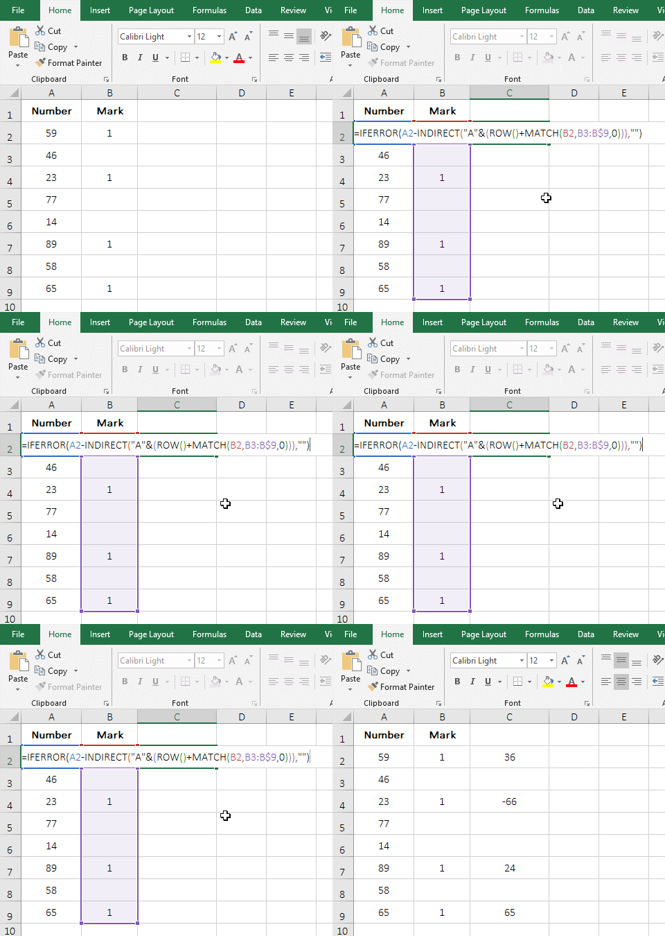
Figure 6

2. Formula =IFERROR(A2-INDIRECT("A"&(ROW()+MATCH(B2,B3:B$9,0))),"") description:

A. ROW() is used to return the row number of the row where the formula is located. When the formula is in C2, it returns 2.

B. MATCH(B2,B3:B$9,0) is used to return the position of mark(ie 1) that is closest from B2 and under B2; the result is 2; B2 is the Lookup_Value, B3:B$9 is the Lookup_Array, and 0 is the exact Match; B2 and B3 are relative references, when dragging down, B2 will become B3, B4, etc., B3 will become B4, B5, etc.; B$9 means absolute reference to column and relative to row, when dragging down, B$9 does not become B10, B11, etc.; B3:B$9 is used because it is always necessary to find the mark in the range from the next cell of the current cell to the last cell.

C. Then INDIRECT("A"&(ROW()+MATCH(B2,B3:B$9,0)) becomes INDIRECT("A"&(2+2)), further calculation becomes INDIRECT("A4"), then use Indirect to return a reference to the string "A4", which returns 23.

D. The formula becomes =IFERROR(A2-23,""), A2 is 59, A2-23 is equal to 36; IfError is the error handling function, if A2-23 returns an error, IfError returns "", otherwise it returns A2-23.

(IV) Subtract one number from all the numbers in the table

1. If you want to subtract 10 from all the numbers in the table. Select cell F2, enter 10, press Enter, select F2 again, press Ctrl + C to copy, select B2, hold down the Shift key, click E9, select B2:E9, right-click the selected area, and select "Paste Special" in the pop-up menu to open "Paste Special" "Window, select "Value" under "Paste", then select "Subtract" under "Operation", click "OK", then all the numbers in the table are reduced by 10; the operation steps are as shown in Figure 7:

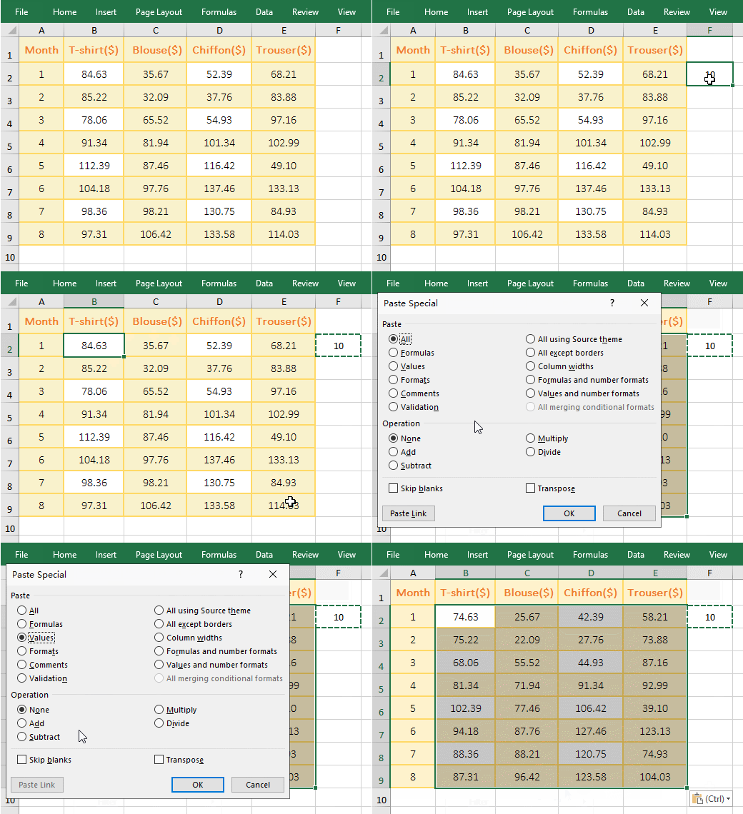
Figure 7

2. If you select "All" under "Paste", the format of the cell F2 where 10 is located will be pasted to B2:E9, that is, the format of B2:E9 is overwritten by F2 format, but "Value" is selected, then just pasting the value will not overwrite the format.