 Office > Excel > Excel 2019 > Content
How to calculate square, cubic, Nth and square root in excel with Powre or SQRT function
There are two methods for calculating the square, cubic, and Nth powers (the power of N) in Excel, one is calculated by the Power function, and the other is calculated by the caret(^); there are three methods for calculating the square root, calculated by the SQRT, Power and caret(^), respectively. When calculating the square of a negative number, if you want to return a negative number, you must bracket the base and the exponent. When calculating the square root with the caret(^), enclose the fraction after the caret.
If you want to calculate the sum of squares, you can use the SumSQ function; if you want to calculate the sum of squares and then square, you can use the SumSQ + Power(or ^) function; if you want to calculate the sum of multiple powers of numbers, you can use Sum + Row function.
I, How to calculate the square, cubic and Nth power in Excel
(I) Calculated by the Excel Power function(Exponential function)
1. Expression: POWER(Number, Power), Number is the base, Power is the exponent.
2. A method for calculating the square, cubic, and Nth powers.
Suppose you want to calculate the square, cubic, and 16th power of 5. Double-click the cell B2, copy the formula =POWER(A2,2) to B2, press Enter, return to 25 that is the square of 5; double-click C2, paste the same formula to C2, change 2 to 3, press Enter, return 125 that is the cubic of 5; double-click D2, paste the same formula to D2, change 2 to 16, return to 1.52588E+11 that is the 16th power of 5; the operation steps, as shown in Figure 1:

Figure 1
(II) Calculated with the caret(^)
^ equivalent to the Power function, also used to calculate the square, cubic and 16th power of 5 as an example. Double-click the cell B2, copy the formula =A2^2 to B2, press Enter, return to 25 that is the square of 5; double-click C2, paste the same formula to C2, change 2 to 3, press Enter, return to 125; then double-click D2, paste the same formula to D2, change 2 to 16, press Enter, and return to 1.52588E+11; the result is exactly the same as the above calculation; the operation steps are as shown in Figure 2:
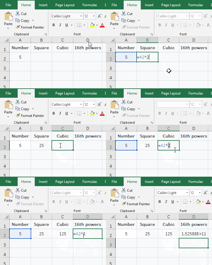
Figure 2
(III) Calculate the square cube of the negative number
1. If you want to calculate the square and cube of -2, return positive and negative numbers, respectively. Double-click the cell B2, copy the formula =A2^2 to B2, press Enter, return to 4; double-click B3, paste the formula =A2^2 into B3, enter the minus sign(-) before A2, press Enter, also return 4; double-click B4, paste formula =A2^2 to B4, and change the formula to =-(A2^2), press Enter, return -4; double-click B5, copy formula =-2^2 to B5, press Enter, return to 4, double-click B6, paste formula =-2^2 into B6, and add brackets to 2^2, press Enter, return -4; double-click C2, copy formula =A2^3 to C2, press Enter, return -8; double-click C3, paste formula =A2^3 to C3, and enter the negative sign before A2, press Enter, return to 8; the operation steps, as shown in Figure 3:
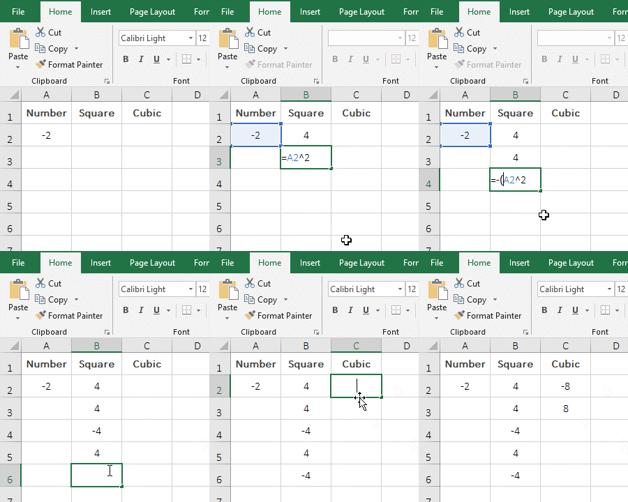
Figure 3
2. The formula =-2^2 returns the square of -2 is 4, because calculation priority of the minus sign(-) is greater than the power(^), that is, first -2 then square; formula =A2^2 and =-A2^2 return 4 is the same meaning; therefore, if the square of the negative number is to return a negative number, you need to enclose the number and power in parentheses, such as =-(A2^2) or =-(2^2).
II, How to calculate square root in Excel
(I) Calculated by SQRT function
1. If you want to calculate the square root of 2 and 3. Double-click cell B2, copy the formula =SQRT(A2) to B2, press Enter, return 1.414213562 that is the square root of 2; select B2, move the mouse to the cell fill handle in the lower right corner of B2, after the mouse becomes bold black plus sign, double-click the left button to return 1.320050808 that is the square root of 3; the operation steps, as shown in Figure 4:
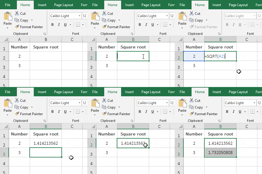
Figure 4
2. If you want the return value to round up to two decimal places, you can select B2 and B3, press the shortcut key Ctrl + 1 to open the "Format Cells" window, select the "Number" tab, and then select the "Number" on the left, enter 2 after the "Decimal places" on the right, click "OK".
(II) Using the Power function to calculate
1. Also take the calculation of square root of 2 and 3 as an example. Double-click the cell B2, copy the formula =POWER(A2,1/2) to B2, press Enter, return to the square of 1.414213562; select B2, move the mouse to the cell fill handle in the lower right corner of B2, after the mouse changes the bold black plus sign, press and hold the left button and drag down, drag to B3, then return the square root 3.73250808; the calculation result of the two numbers is consistent with the result calculated by the SQRT function; the operation steps, as shown in Figure 5:

Figure 5
2. Calculate the square root with the Power function, just write the exponent as a fraction. For example, calculates the square root of 2, the exponent is written as 1/2, as the formula =POWER(A2,1/2).
(III) Calculated with the caret(^)
1. Also take the calculation of square root of the 2 and 3 as an example. Double-click the cell B2, copy the formula =A2^(1/2) to B2, press Enter, return to the square root 1.414213562; return the square of 3 with the method of dragging down, the result is 1.732050808; the results of the square root are also the same as that calculated by the above two methods; the operation process steps are as shown in Figure 6:
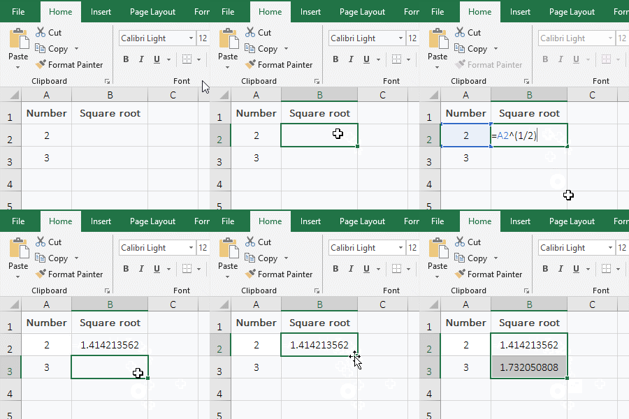
Figure 6
2. Calculate the square root with the caret(^) and write the exponent as a fraction and enclose the fraction in parentheses, otherwise, an error will occur; for example: =A2^1/2 will be resolved to the 1th power of A2 then divide by 2, not the square root of A2.
Hint: Negative numbers cannot be calculated square root. Any of the above methods will not work. No matter which method is used, the value error #NUM! will be returned.
III, How to calculate N-th root in Excel
1. Calculated with ^
If you want to calculate the 8th root of 65536 and 2. Double-click the cell B2, copy the formula =A2^(1/8) to B2, press Enter, return to 4 that is the 8th root of 65536; then double-click the cell fill handle of B2 to return the 8th root of 2, the result is 1.090507733; the operation steps are as shown in Figure 7:
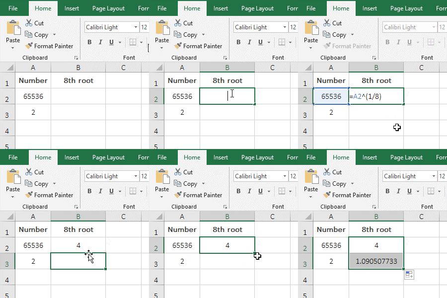
Figure 7
2. Using the Power function to calculate
Also take the example of calculating the 8th root of 65536 and 2. Double-click the cell B2, copy the formula =POWER(A2,1/8) to B2, press Enter, return to 4; then return 1.090507733 with the method of dragging down; the result of the two numbers is exactly the same as that calculated by ^; the operation process steps are as shown in Figure 8:
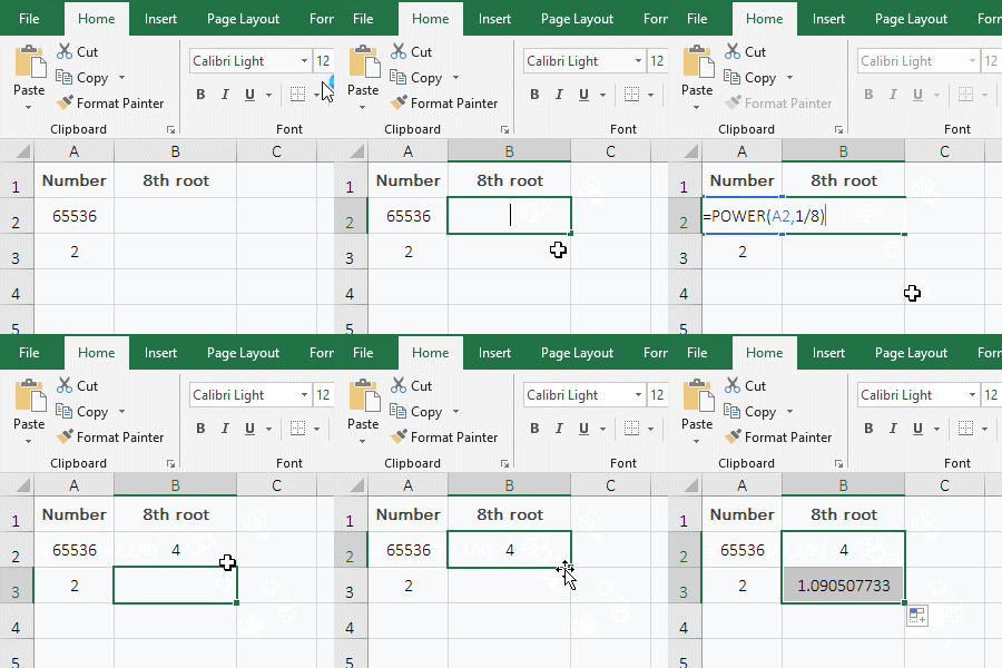
Figure 8
IV, Excel calculates the sum of squares and multiple powers(Power is an array)
(I) How to calculate sum of squares in Excel
1. If you want to calculate the sum of the squares of A2 to C2. Double-click cell the D2, copy the formula =SUMSQ(A2:C2) to D2, press Enter, return the result 529; the operation steps are as shown in Figure 9:
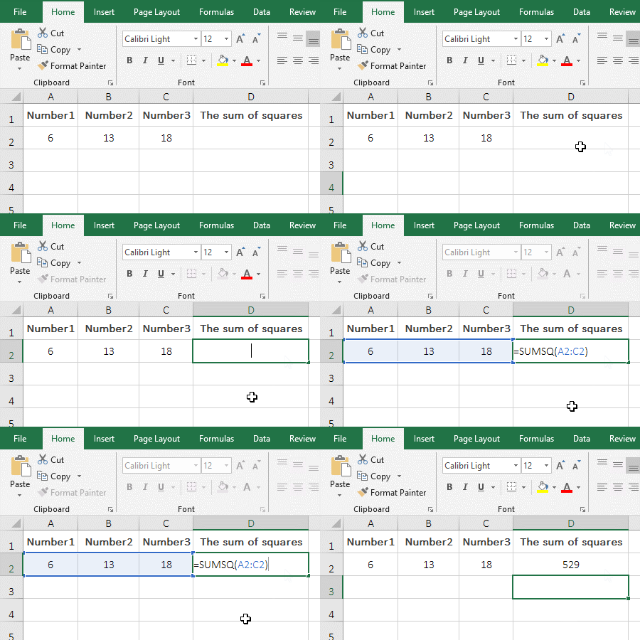
Figure 9
2. Description:
A2:C2 means to reference the three cells A2 to C2 in the formula =SUMSQ(A2:C2). The SumSQ function is used to calculate the sum of squares, it can have up to 255 argument, the argument can be numbers, arrays or references to cells. If there are texts in the arguments that cannot be converted to numeric values, an error will be returned.
(II) How to calculate the sum of multiple powers(Power is an array)
1. If you want to calculate the sum of powers 1 to 10 of 2 and 3. Double-click B2, copy the formula =SUM(A2^ROW(1:10)) to B2, press Ctrl + Shift + Enter, return 2046 that is the sum of powers 1 to 10 of 2; drag down to return 265,716 that is the sum of powers 1 to 10 of 3; the operational steps, as shown in Figure 10:
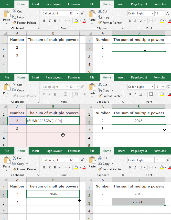
Figure 10
2. Formula =SUM(A2^ROW(1:10)) explanation:
1. ROW(1:10) returns a value from 1 to 10 as an array, which returns {1;2;3;4;5;6;7;8;9;10}.
2. A2 is 2, the formula becomes =SUM(2^{1;2;3;4;5;6;7;8;9;10}), and then each element in the array is taken as the exponent of 2 And calculate, then the formula becomes =SUM({2;4;8;16;32;64;128;256;512;1024}), and finally adds each element in the array.
(3) Calculate square root after square sum
1. If you want to calculate the sum of squares in column A, then calculate square root. Double-click the cell B2, copy the formula =SUMSQ(A2:A6)^(1/2) to B2, press Enter, return to 13.52774926; the operation steps are as shown in Figure 11:
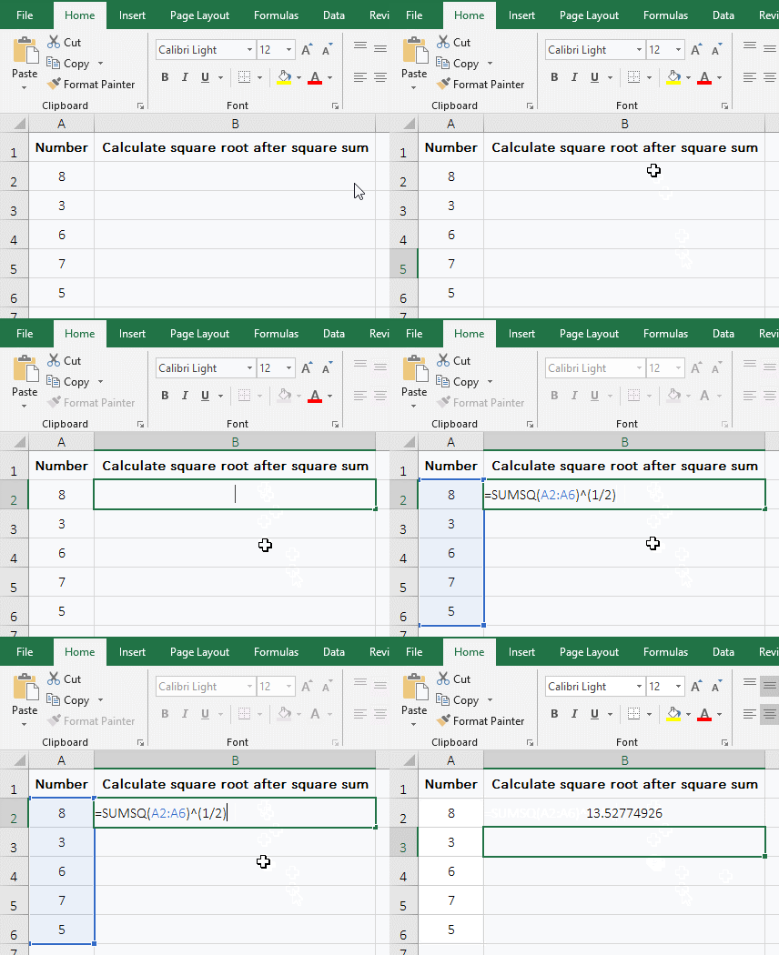
Figure 11
2. Formula description:
First, calculate the sum of the squares in A2:A6 with the SumSQ function, the result is 195, and then calculste the square of 195, the result is 13.52774926.
V, How to calculates the sum of squares of deviations in Excel
1. If you want to calculate the sum of squares of deviations in column A. Double-click the cell B2, copy the formula =DEVSQ(A2:A6) to B2, press Enter, return the calculation result 26.8; the operation procedure is as shown in Figure 12:
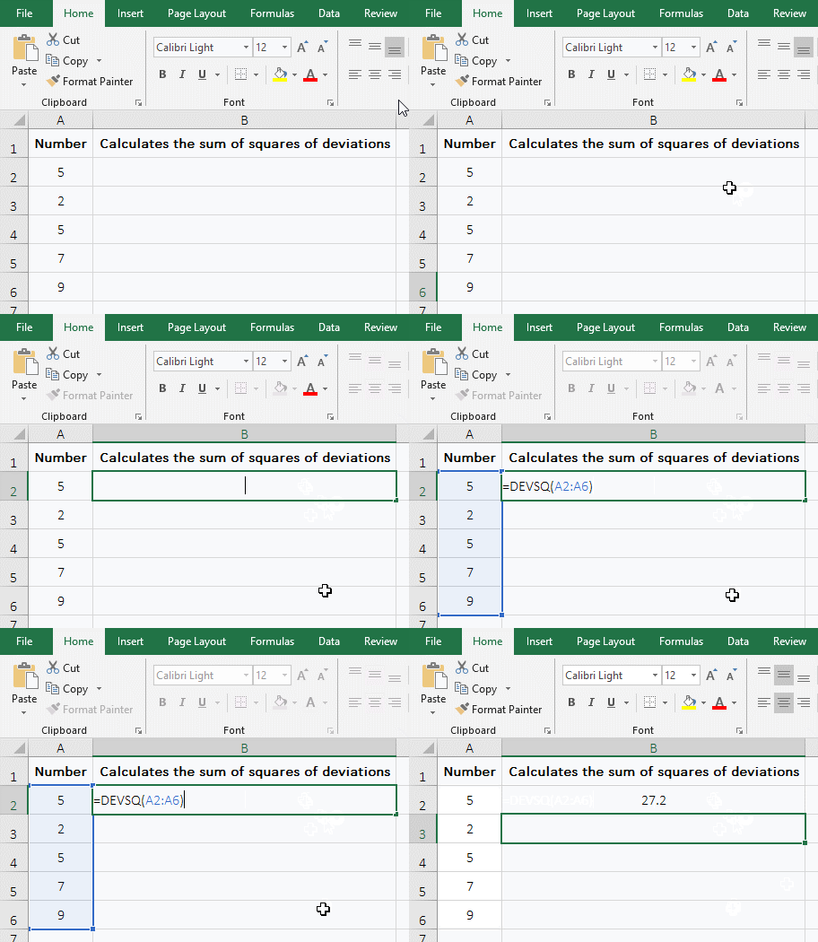
Figure 12
2. Description:
The DEVSQ function is used to calculate the sum of the squares of the difference(ie, the data deviation, also known as the dispersion) between each data point and the data mean point. It must have at least one argument and a maximum of 255 arguments.
-
Related Reading
- Excel CountA and CountBlank function usage examples(
- 8 examples of Excel Match function, include it and S
- How to use offset function in excel, include it and
- Excel SumProduct function(multiple criteria, with if
- Excel left function usage(8 examples, with Sum+Value
- How to use Average function in excel(combine with if
- Excel If function examples, include if statement nes
- How to use Excel address function(7 examples, with I
- Excel SumIf function with ?/*, Average and array mul
- How to use Excel subtotal function(combine it with O
- How to use excel aggregate function(ignore error val
- How to use Excel find function(9 examples, include f