Excel row function examples, with Rows, Row(A:A), Row(1:1) and add even or odd rows

The Row function is used to return the row number of a reference cell or a range of cells in Excel. If the argument is omitted, it will return the row number of the row in which the formula is located. The Rows function is used to return the number of rows of the array or cells that are referenced, there is only one parameter and cannot be omitted.

Row functions is often used in combination with Index, Small, Match, Indirect, OffSet, If, SumProduct, CountA, etc. For example, the Row + Indirect + CountA combination returns all non-null cells as an array, SumProduct + Row + Mod combination adds even or odd rows. Alternatively, if you want to return a reference to a column, you can use Row(A:A); to return a reference to a row, you can use Row(1:1).

I, Excel Row function and Rows function syntax

1. Expression: ROW([reference])

2. Expression: ROWS(Array)

3. Description:

A. Row function is used to return the Row_Num of a cell or cell range referenced. The argument Reference is optional, if omitted, the Row_Num in which formula is located is returned. If Reference is a vertical reference to a range of cells (such as A1:A9), the Row function returns the row number of all referenced cells as an array. You can see when pressing F9 or Row(A1:A9) as the criteria of If, as shown in the following example; Reference cannot refer to multiple ranges at once.

B. Rows function is used to return the number of rows referenced. The argument Array is an array or a reference to a range of cells and cannot be omitted.

II, Excel row function examples

(I) Returns the row number of the row in which the formula is located

1. Select cell A1, enter the formula =ROW(), press Enter, return 1; select A1, move the mouse to the cell fill handle in the lower right corner of A1, and after the mouse becomes the bold black plus, press and hold the left button and drag down, the Row_Num of rows that are passed through are returned; the operation process steps, as shown in Figure 1:

Figure 1

2. Description: The formula =ROW() omits the argument Reference and returns the Row_Num of rows in which the formula is located.

(II) Return the Row_Num of the specified row

Select cell B1, enter the formula =ROW(A5), press Enter, return to the Row_Num 5 of of A5; the operation steps are as shown in Figure 2:

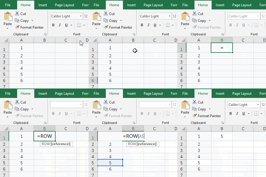
Figure 2

(III) A vertical reference to a range of cells and returns the array

1. If you want to return all the row numbers of A1:A5. Double-click cell B1, copy the formula =IF(ROW(A1:A5)>=3,A1:A5,0) to B1, press Ctrl + Shift + Enter, return 0; hold down the Alt key and press M And V separately, open the "Evaluate Formula" window, press Enter to evaluate, then ROW (A1:A5) returns an array of 1 to 5; the operation steps, as shown in Figure 3:

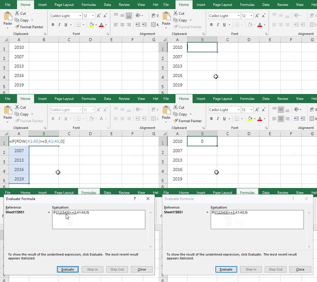
Figure 3

2. Formula description:

A. The formula =IF(ROW(A1:A5)>=3,A1:A5,0)) is an array formula, so press Ctrl + Shift + Enter.

B. ROW(A1:A5)>=3 is the criteria of If, ROW(A1:A5) returns the row numbers of A1:A5 as an array, that is, {1;2;3;4;5}. When excuting, all elements in the array will be taken out and are compared to 3, if it is greater than or equal to 3, return True, otherwise return False; finally return {FALSE;FALSE;TRUE;TRUE;TRUE}; returns the element in A1:A5 when all elements in the array are true, so returns 0.

(IV) Refer to a column Row(A:A) and a row Row(1:1)

1. Reference a column; select cell B1, enter formula =ROW(, click Column_Num A of the first column, then A:A are automatically inputted, then enter the right parenthesis ), press Enter, return 1. Reference a row; select currently B2, enter =ROW(, click the Row_Num 1 of the first row, then 1:1 are automatically input, then enter the right parenthesis ), press Enter, return to 1; the operation steps, as shown in Figure 4:

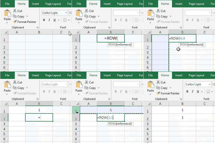
Figure 4

2. Formula description:

A. After input =ROW(, to refer to that column or that row, click the corresponding Column_Num or Row_Num, in addition, you can also enter the Column_Num or Row_Num; if you refer to the second column, the formula is =ROW(B:B); Referring to the second row, the formula is =ROW(2:2).

B. In addition, the formula =ROW(A:A) can also be changed to =ROW($A:$A), the formula =ROW(1:1) can also be changed to =ROW($1:$1), that is, add the absolute quotation $ before the Dolumn_Num and the Row_Num to change the relative reference to an absolute reference.

3. If you want to return an array, you also need to put =ROW(A:A) or =ROW(1:1) in a function whose argument is a reference. For example, if =ROW(A:A) is inserted in the Index function, the formula becomes =INDEX(ROW(A:A),2), copy the formula to the cell B1, press Ctrl + Shift + Enter, return 2; Hold down the Alt key, press M and V respectively, open the "Evaluate Formula" window, press Enter to evaluate, then return all the row numbers of column A; the operation process steps, as shown in Figure 5:

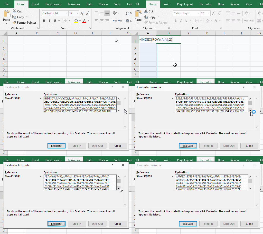
Figure 5

The formula =INDEX(ROW(A:A),2) is used to return a reference to a cell specified by a row number in the column A, ROW(A:A) is the reference to a cell range, 2 is the

The formula =INDEX(ROW(A:A),2) is used to return a reference to a cell specified by a row number in the column A, ROW(A:A) is the reference to a cell range, 2 is the Row_Num, the formula omits the Column_Num, the meaning of the formula is: return the Row_Num of the second row in column A, so return 2.

(V) Use the function in the argument(Row + Indirect + CountA)

1. Double-click cell E2, copy the formula =ROW(INDIRECT("1:"&COUNTA(D:D))) to E2, press Enter, return to 1; select E2, hold down the Alt key, and press M and V in sequence, open the "Evaluate Formula" window, press Enter three times, return ROW($1:$7); the operation steps, as shown in Figure 6:

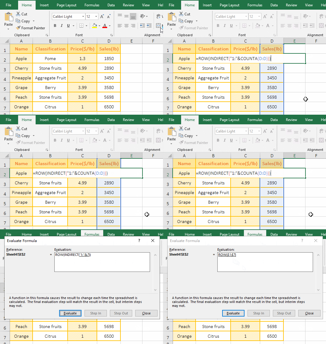
Figure 6

2. The formula =ROW(INDIRECT("1:"&COUNTA(D:D))) description:

A. COUNTA(D:D) is used to count the number of non-empty cells in column D, it returns 7; then INDIRECT("1:"&COUNTA(D:D)) becomes INDIRECT("1:"&7), further calculation change to INDIRECT("1:7"), then return a reference to the text "1:7" with the Indirect function, which returns $1:$7.

B. The formula becomes =ROW($1:$7), andy returns finall an array of 1 to 7 as an array. You also need to put =ROW($1:$7) in the Index function to return the array.

III, The examples of Excel Rows function

(I) The argument is an array

1. Double-click cell A1, copy the formula =ROWS({5,21,8,13,4,59}) to A1, press Enter, return to 1; double-click A1 again, change the second and fourth comma(,) to a semicolon(;) in the formula, press Enter, return to 3; the operation steps, as shown in Figure 7:

Figure 7

2. Formula description:

The array in the formula =ROWS({5,21,8,13,4,59}) has only one row, and the array in the formula =ROWS({5,21;8,13;4,59}) has three rows, the rows are separated by semicolons, and elements are separated by commas in array; the first formula has only commas without a semicolon, so there is only one row; the second formula has two semicolons, so there are three rows.

(II) The argument is the reference to a cell range

1. Double-click B1, copy the formula =ROWS(A1:A5) to B1, press Enter, return to 5; enter =ROWS( in B2, click the Column_Num A of the first column, then automatically enter A:A, then enter right parenthesis ), press Enter to return to 1048576; the operation steps are as shown in Figure 8:

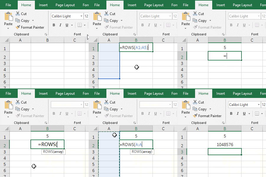
Figure 8

2. Formula description:

The formula =ROWS(A1:A5) returns the number of rows of A1:A5, A1 to A5 are 5 rows, so 5 is returned; the formula =ROWS(A:A) returns the number of rows in column A, and the column A has 1048576 rows.

IV, The extended application examples of Excel Row function

(I) SumProduct + Row + Mod combination adds even rows or odd rows

1. If you want to return separately the sum of the even and odd rows of Sales. Double-click cell D8, copy the formula =SUMPRODUCT((MOD(ROW($2:$7),2)=ROW(A1))*D$2:D$7) to D8, press Enter, return to 12970; then double-click D9, copy the formula =SUMPRODUCT((MOD(ROW($2:$7),2)=0)*D$2:D$7) to D9, press Enter, return to 10998; the operation steps are as shown in Figure 9:

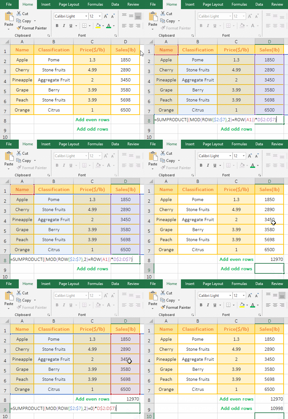
Figure 9

2. Add the even rows formula =SUMPRODUCT((MOD(ROW($2:$7),2)=ROW(A1))*D$2:D$7) explanation:

A. ROW($2: $7) returns the Row_Num of 2 to 7 rows as an array, then MOD(ROW($2:$7),2) becomes MOD({2;3;4;5;6;7},2), then take the first element 2 from the array, and then modulo with 2, the result is 0; then take the second element 3 from the array, and then modulo with 3, the result is 1; the other and so on, and finally returns {0;1;0;1;0;1}.

B. ROW(A1) returns the Row_Num 1 of A1; then MOD(ROW($2:$7),2)=ROW(A1) becomes {0;1;0;1;0;1}={1}, further calculations, take each element from the array and compare it to 1, if it is equal, it returns True, otherwise it returns False, and finally returns {FALSE;TRUE;FALSE;TRUE;FALSE;TRUE}.

C. D$2:D$7 returns the values in D2 to D7 as an array, which returns {0;2890;0;3580;0;6500}.

D. The formula becomes =SUMPRODUCT({FALSE;TRUE;FALSE;TRUE;FALSE;TRUE}*{0;2890;0;3580;0;6500}), further calculation, multiplying the corresponding elements of the two arrays, then add all the products; when multiplied, True turns to 1, False turns to 0, and finally returns the summation result 12970.

Hint: The first row(D2) in D2:D7 is the starting row that is added in the above formula. If the first row of the table is the starting row, it is the sum of the odd rows.

3. Add the odd rows formula =SUMPRODUCT((MOD(ROW($2:$7),2)=0)*D$2:D$7) explanation:

The formula that add the odd rows is the same as the formula that add the even rows, just change MOD(ROW($2:$7),2)=ROW(A1) to MOD(ROW($2:$7),2)=0, because the modulus (ie the remainder) ) is 0 for odd rows, where the summation region D2:D7 also starts with D2.