How to use Excel product function(10 examples, with multiply and divide in formula and exponential)

The calculation of multiplication can be either a Product function or an asterisk * in Excel, but they differ. The Product function not only takes a single value as a argument, but also takes an array and a reference to cells as arguments, for example, to calculate the product of all values in A1 to A6, it does not need to be written one by one, just write A1:A6; and it can be written only one by one with an asterisk. In addition, how to divide in excel? There are two ways to calculate the division, one is to use the Product function, and the other is to use the slash(/), the difference is the same as the calculation multiplication.

You usually encounter all the numbers that are multiplied or divided by a number in the multiplication and division calculation process. They are implemented by the functions provided by Excel, and can also be implemented by Excel multiply formula or division formula. The difference is: one is modified in the original data and the other is generating new data.

I, Excel product function syntax

1. Expression: PRODUCT(Number1, [Number2], ...)

2. Description:

A. Product function can only have a maximum of 255 Number.

B. If the logical values(True and False) are directly used as arguments to the Product function, True is converted to 1, and False is converted to 0; if the logical values are in an array or cell to be referenced, they are ignored.

C. If the array or cell range to be referenced contains spaces or text, they are also ignored when evaluated.

II, The examples of Excel Product function(Multiply function in Excel)

(I) Examples of multiplication of the numbers in two columns

1. If the turnover is required. Double-click the cell E2, copy the formula =PRODUCT(C2,D2) to E2, press Enter, return to 2405; select E2, move the mouse to the cell fill handle in the lower right corner of E2, after the mouse becomes the bold black plus(+) , double-click the left button to return the remaining turnover; the operation process steps, as shown in Figure 1:

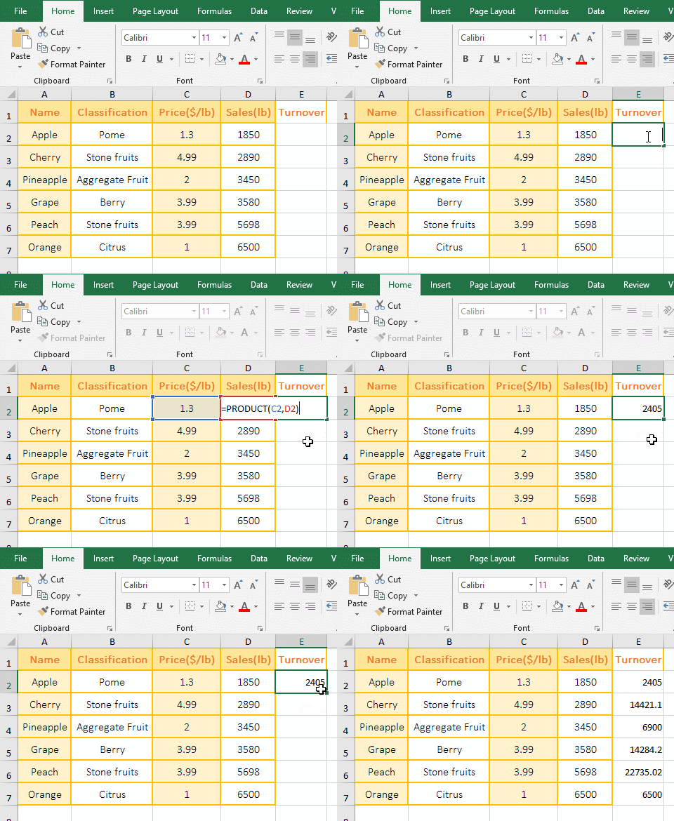
Figure 1

2. Description: C2 and D2 are the cells to be referenced in the multiplication formula =PRODUCT(C2,D2), which means multiplying the numbers in C2 and D2.

(II) True and False are different value in cells, arrays or as arguments directly

1. Select the cell B1, enter the formula =PRODUCT(A1:A3), press Enter, return to 3. Double-click B2, copy the formula =PRODUCT({3,TRUE,FALSE}) to B2, press Enter, return 3; Double-click B3, copy the same formula to B3, and remove the two braces, press Enter, return 0; the operation steps, as shown in Figure 2:

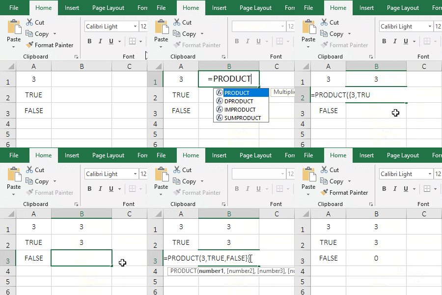
Figure 2

2. Formula description:

A. The multiplication formula =PRODUCT(A1:A3) and =PRODUCT({3,TRUE,FALSE}) both return 3, indicating that the logical values?(True and False) are ignored in both the referenced cells and the array.

B. Multiplication formula =PRODUCT(3,TRUE,FALSE) returns 0, indicating that True and False are used as arguments directly, True is converted to 1, and False is converted to 0.

(III) The argument is the cell range to be referenced

1. If the product of the two columns A and B is required. Double-click the cell C1, copy the formula =PRODUCT(A1:A5,B1:B5) to C1, press Enter, return to 9.90; the operation steps are as shown in Figure 3:

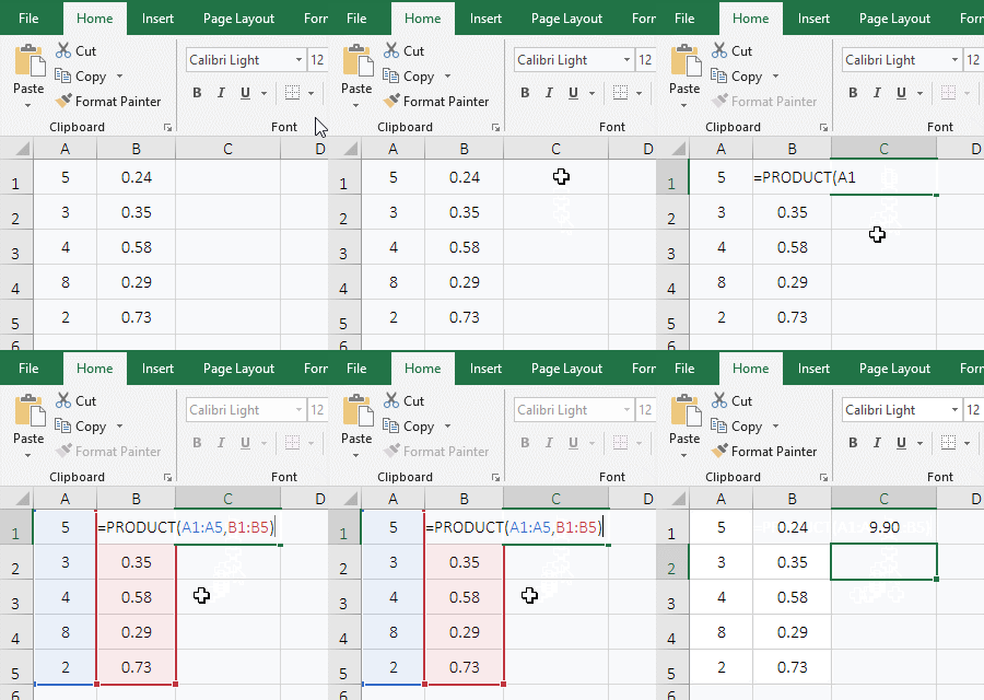
Figure 3

2. Formula description:

Multiplication formula =PRODUCT(A1:A5,B1:B5) Multiplies all the numbers in A1:A5 and B1:B5, ie A1 * A2 * A3 * A4 * A5 * B1 * B2 * B3 * B4 * B5.

III, How to multiply in Excel with *

1. Also take the calculation of turnover as an example. Select cell E2, enter formula =C2*D2, press Enter, return to 2405; select E2 again, click the cell fill handle of E2 to return the remaining turnover; the operation steps are as shown in Figure 4:

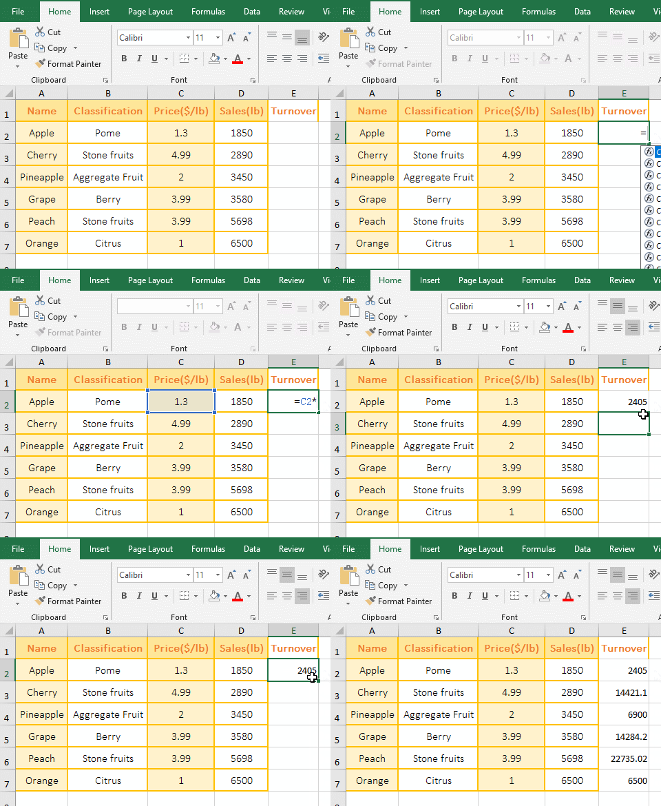
Figure 4

2. When calculating multiplication with *, you cannot do this =(C2:C7)*(D2:D7) to return the product of two columns of numbers, so that only the product of C2 * D2 can be returned.

IV, How to divide in Excel

There is no function to calculate directly the division in Excel. The division calculation requires the multiplication function Product, and can also be calculated with a slash(/). The following is their calculation method.

(I) How to divide with the Product function in Excel

Double-click the cell C1, copy the formula =PRODUCT(A1/B1) to C1, press Enter to return to 20.83; select C1 and double-click the cell fill handle of C1 to return the remaining results; the operation steps are as shown in Figure 5:

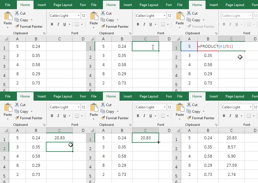
Figure 5

(II) How to divide with slashes(/) in Excel

Select the cell C1, enter the formula =A1/B1, press Enter, return to 20.83; select C1 again, and double-click the cell fill handle of C1 to return the result of dividing the remaining values; the operation steps are as shown in Figure 6:

Figure 6

Tip: The Excel division calculation will round up to multiple decimals by default. If you want to round up to two decimals, you can press Ctrl + 1, open the "Format Cell" window, select "Number" Tab, then select "Number" on the left, then enter 2 to the right of "Decimal Places" on the right, click "OK".

V, Multiply or divide all the numbers in the table by a number in Excel

(I) Multiply all the numbers in the table by a number

If you want to multiply all sales in the table by 0.2. Select cell E2, enter 0.2, press Enter to exit the input state, select E2 again, press Ctrl + C to copy; select D2:D7, right click on them, select "Paste Special" in the pop-up menu, select "Multiply" under "Operation" in the "Paste Special" window, click "OK", then all sales in the table are multiplied by 0.2; the operation steps, as shown in Figure 7:

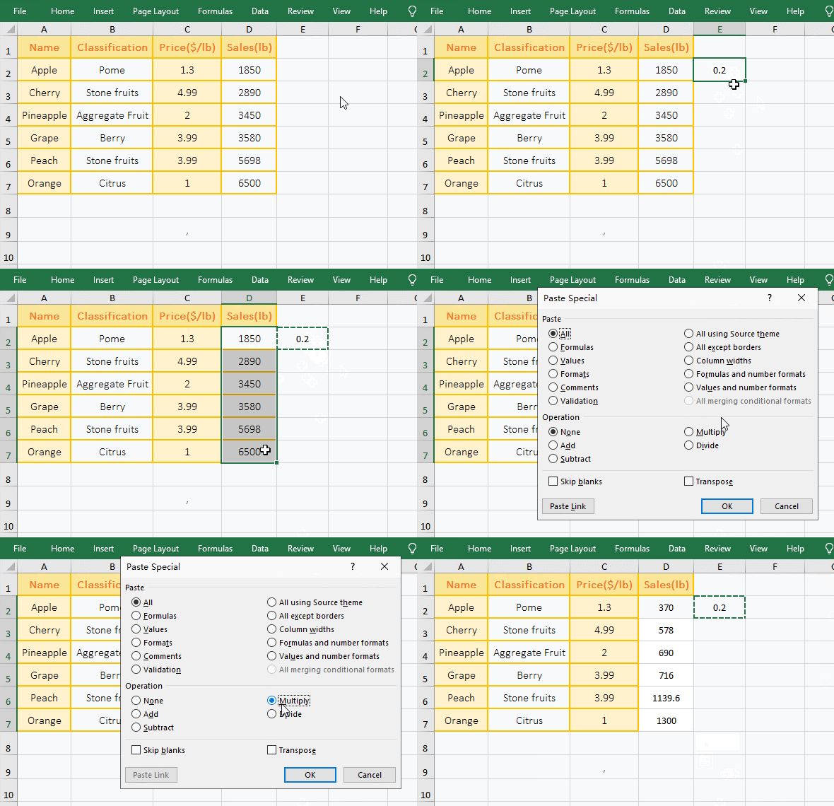
Figure 7

(II) Divide all the numbers in the table by one number

If you want to divide all sales in the table by 2. Select E2, enter 2, press Enter, exit the input state, select E2 again, press Ctrl + C to copy; select D2:D7 and right click on them, then select "Paste Special", select "Divide" under "Operation" in the window that has been opened, click "OK", then all sales in column D are diveded by 2; the operation steps are as shown in Figure 8:

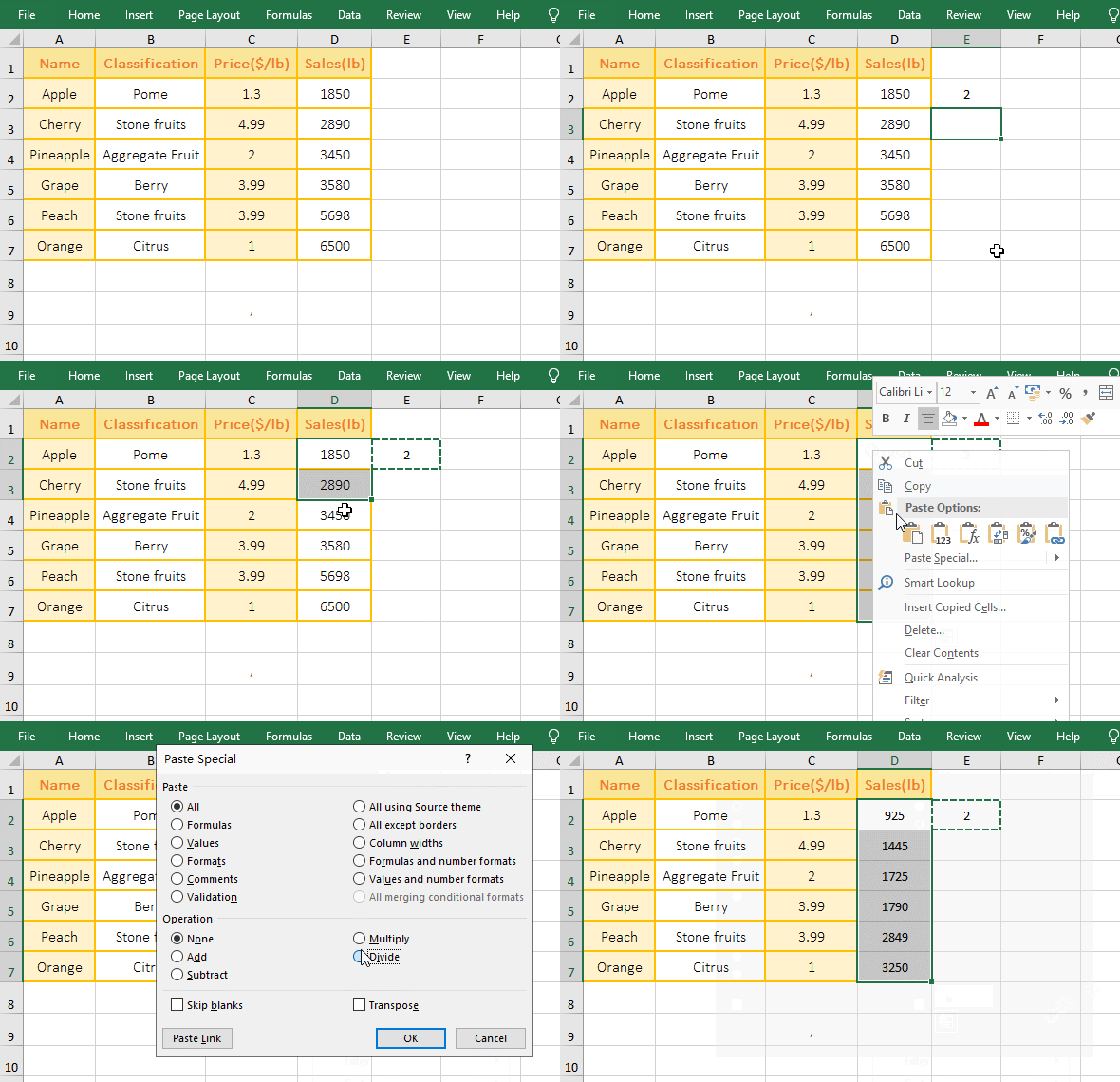
Figure 8

VI,  The extension application examples of Excel Product function

(I) If + Product function combination realizes price increase according to criteria

1. If you want to increase the price of fruit by less than $3 by 10%. Double-click the cell E2, copy the formula =IF(C2<3,PRODUCT(C2,(1+10%)),C2) to E2, press Enter, return to 1.43, because 1.3 in C2 meets the criteria, so increased the price; Select E2 again, and double-click the cell fill handle of E2 to increase the price of the remaining price; the operation steps are as shown in Figure 9:

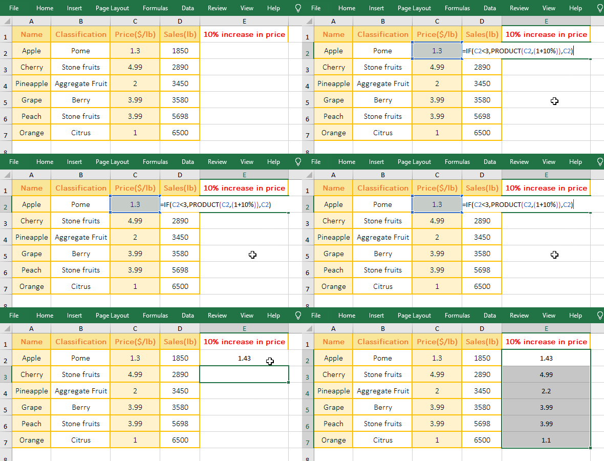
Figure 9

2. Formula =IF(C2<5,PRODUCT(C2,(1+10%)),C2) explanation:

A, C2<5 is the criteria of If; if the criteria is true, the price is increased by 10% with PRODUCT(C2,(1+10%)), that is, the value 1.3 in C2 is multiplied by (1+10%); otherwise, it returns to C2; since the value in C2 is 1.3, the criteria is met, so PRODUCT(C2,(1+10%)) is returned, the result is 1.43.

B. When the formula is in C3, C3(4.99) > 3, the criteria is not met, so the value in C3 is returned; the others and so on.

3. If you want to return only the prices that are increased, you can use this formula =PRODUCT(IF(C2<3,C2,0),1+10%), as shown in Figure 10:

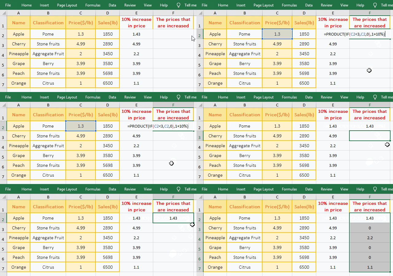
Figure 10

(II) Array and reference to cells exponential operation

1. Array exponential operation; double-click the cell B2, copy the formula =PRODUCT({5,3}^{1,-1}) to B2, press Enter, return 1.666666667. Reference to the cell exponential operation; double-click C2, copy the formula =PRODUCT((A2:A3)^{1,-1}) to C2, press Ctrl + Shift + Enter, return to 1; the operation steps are as shown in Figure 11:

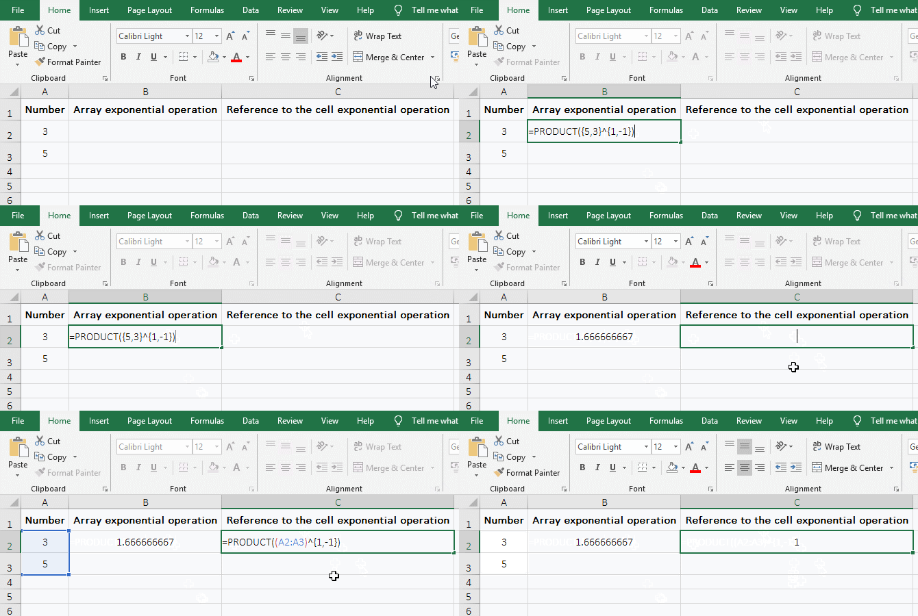
Figure 11

2. Formula description:

A. There are two arrays in the formula = PRODUCT({5, 3}^{1,-1}), the first is the base array, the second is the exponential array; when calculating, first, takes out 5 from the base array, takes 1 from the exponential array, that is, calculate the 1st power of 5, the result is 5;  Second, takes 3 from the base array, and takes -1 from the exponential array, that is, calculates the -1 power of 3, that is, 1/3, the result is 0.333333333333333; finally multiply the results of the two calculations, that is, 5 * 0.333333333333333 is equal to 1.666666667.

B. The formula =PRODUCT((A2: A3)^{1,-1}) is an array formula, so press Ctrl + Shift + Enter; A2:A3 returns the values in A2 and A3 as an array, ie {5;3}, then the formula becomes =PRODUCT({5;3}^{1,-1}), just like the array {5,3} is written directly into the formula, but the calculation method is different. 

When calculating: 

First, takes 5 from the base array, then takes 1 and -1 from the exponent array, then calculate the 1th power and the -1 power of 5, and the result is 5 and 0.2; 

Second, takes 3 from the base array, takes 1 and -1 from the exponent array, then calculate the 1st power and -1 power of 3, and the result is 3 and 0.333333333333333; then the formula becomes =PRODUCT({5,0.2;3,0.333333333333333}), and finally all elements in the array are multiplied and the result is 1.